5 Programming work flows
When considering a programmatic solution to a problem, all but the simplest scripts will require some consideration as to the structure of the code. Some of the main paradigms are now discussed. Given the abstract nature of the terminology, examples will be discussed before defining the new terms, unlike the previous sections that began with definitions which were then illustrated by examples.
5.1 Structured Programming
Given the simplicity of importing code from one script file into another, a typical coding solution would span multiple files from several directories. Take for example the bookdown R package, which has been used to construct this guide. This directory has been copied from its github site where an interested reader can go to examine this directory for themselves.
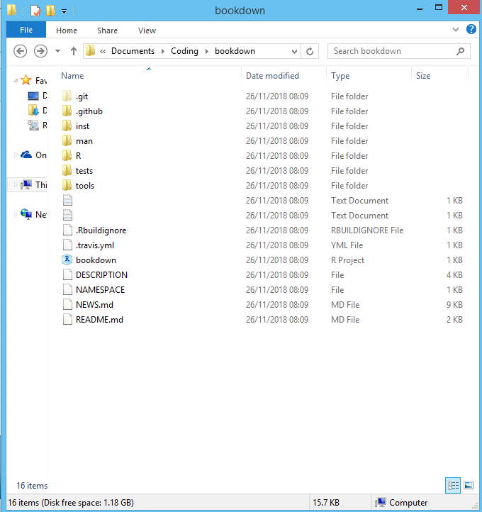
Figure 5.1: The bookdown R package file structure
The files that can be seen in the current directory set the context for the package, for example:
- the
README.mdfile summarises the package contents and where to find more information. - the
bookdown.Rprojfile is a project file that can be clicked to open the solution in RStudio quickly. - the unnamed text documents (
.gitignoreand.gitattributes) contain setting relevant to version control.
The folders then contain the code, for example:
- the
Rdirectory contains several.rfiles that comprise the bookdown package functionality. - the
manfolder contains files that describe the code’s functionality (ie the manual). - the
instdirectory contains examples, templates and further resources that use theRfunctions. - the
testsdirectory includes automated tests that confirm the functionality of theRcode is performing as expected.
Structuring a coding solution as a collection of files in this way has several advantages. Code that is used several times (eg making a connection to a database) can be defined in one place and imported where relevant. This saves on repetition, and should this functionality need to be updated (eg for a new database location/password), the code can be altered once without the need to do a find and replace across everything. This concept is referred to as code abstraction.
Seperating different elements this way also better enables automated testing to be performed. For each component, complimentary test files can be written that assert whether the components perform as they are expected to. Multiple tests can be written for a given function, and should the code be updated, the current tests can be run to check whether they all still pass (or not). Some development approaches reverse this order. Following a Test-driven development cycle would require the tests to be written first and the components second, and then its code is refactored until the tests pass.
5.2 Object-oriented Programming (OOP)
Let us consider the need to code for a simple rectangle. We could just save the length and width variables for our new rectangle and calculate length * width as necessary to know its area. However, for more complicated objects, such as Policyholder or Pensioner, their properties may be more than simple dimensions, and their methods would certainly be more than simple multiplication.
To demonstrate how to tackle this complexity, we can define a Rectangle class of object that has length and width properties, as well as an area method.
# S3 OOP - other options exist
Rectangle = function(len=1, wid=1) {
  #define class and its properties
  this <- list(
    length = len,
    width = wid
  )
  #define class name
  class(this) <- append(class(this), "Rectangle")
  return(this)
}

#define class functions
area = function(obj) {
  UseMethod("area", obj)
}
area.Rectangle = function(obj) {
  return( obj$length * obj$width )
}

#use an instance of this new class
rectangle1 <- Rectangle(2,3)
area(rectangle1)
# [1] 6

rectangle1$length
# [1] 2
The code begins by defining our Rectangle class, and its two main properties. Class names typically begin with a capital letter, and its definition here includes a default value of 1 for each of its properties. The class is created with len and wid variables, but the data is actually stored in the length and width variables. The area function is then defined and appended to the Rectangle class. R isn’t an OOP language by nature, hence the verbosity of this code, and the need for utlities such as class(this) and UseMethod to get the Rectangle class defined.
Once the class is defined, it can then be used. We create an instance of the Rectangle class called rectangle1 that has a length of 2 and a width of 3. Applying our area method yields the eventual result that the area of rectangle1 is 2 * 3 = 6.
What if we now wanted to define a Square class? We could copy and paste the Rectangle code and change the name and settings so that only one variable is required to create a Square and its area is simply the one variable squared. Or we could use the Rectangle class itself.
#define a new class using an existing class
Square <- function(len=1) {
  this <- Rectangle(len,len)
  class(this) <- append(class(this),"Square")
  return(this)
}

square1 <- Square(4)
area(square1)
# [1] 16
square1$length
# [1] 4
The Square class is exactly the same as the Rectangle class, except that we can create an instance of it with only one variable. Were we to add a perimeter method to the Rectangle class, then the Square class will also acquire this functionality when the code is re-run.
Now for the terminology. We defined a class called Rectangle that had two attributes and one method. These properties were encapuslated into the class definition, ie the methods and data they need are bound up together into a black-box that is our Rectangle class. Having an input len variable define an interior length variable allows for initial data validation to be performed (excluded here), and for the interior variable to remain private and/or protected from the rest of the code. The rectangle1 object was then instantiated from the Rectangle class.
We then later defined a Square class using inhertiance - the Square class inherited the functionality of Rectangle. A heirachy thus forms, where child classes inherit the properties of their parents. Child classes can have several parents.
Had we considered more shapes, like a Circle or a Triangle, we could have instead started with an interface that defined the properties that each descending child class should have, namely area and perimeter. This is polymorphism (Greek for “many forms”), where one interface defines the properties that each child should have, and each child then implements each property in its own way (either as pi * r^2 or as 0.5 * base * height).
Object design is a topic in itself, in that there are certain design patterns that have been discussed extensively in the literature as a typical way of solving common programming problems.
5.3 Functional Programming (FP)
Whilst OOP focuses on objects, Functional Programming (FP) focuses on functions. FP is therefore a way of writting code that uses functions as its building blocks, without leading to any changes in the rest of the code elsewhere. R has functional programming capabilities, as does the popular tidyverse library, so this programming style would complement this environment well.
Whilst the function variable type has already been discussed in the fundamentals section, there are some further concepts that FP employs.
5.3.1 Recursive Functions
Functions can be defined recursively, where a function is defined using itself within its definition.
# factorial implementation using a for loop
factorial <- function(n){
  n_factorial <- 1
  for(i in 2:n){
    n_factorial = n_factorial * i
  }
  return(n_factorial)
}

# factorial implementation using recursion
recursive_factorial <- function(n){
  if(n == 1){
    # terminating condition
    return(1)
  } else {
    # recursive condition
    return( n * recursive_factorial(n-1) )
  }
}

recursive_factorial(4) == factorial(4)
# [1] TRUE
The recursive_factorial function performs the same task as the original factorial function. However, whilst the latter uses a for loop to calculate the factorial of the input, the former simply calls itself again. A key element of recursive functions therefore is that they have a terminating condition, otherwise this self-referntial loop would continue indefinitely. Once the final recursive_factorial function is called with n = 1, this function will then return 1, and all the interim function calls would then evaluate to multiply this with their own interim values of n, eventually completing the n! calculation.
Using recursion can be seen as a clean way to implement a function, but it may lead to slower code as it can take more time to call a function than to execute a simple statement in a loop. However some algorithms, such as that for the Fibonacci sequence, only have recursive definitions.
fibonacci <- function(n){
  if(n < 2){
    return(n)
  } else {
    return( fibonacci(n-1) + fibonacci(n-2) )
  }
}

# print the first 5 fibonacci numbers
for(i in 1:5) print(fibonacci(i))
# [1] 1
# [1] 1
# [1] 2
# [1] 3
# [1] 5
5.3.2 Anonymous Functions (aka Lambda Expressions)
Functions we have encountered until now are known as named functions. There is another type of functions which has significant importance in functional programming, known as anonymous functions (in R and other Lisp inspired languages), or lambda functions (Python) or lambda expression (C# and Java). Anonymous functions can be simply defined as functions not assigned to any object. R is one of the few languages which mantains the same syntax for named and anonymous functions: they are both defined with the previously seen function(arguments){function body} structure.
# named function example
times2 <- function(x){x * 2}
times2(2)
# [1] 4

# Anonymous function implementation
(function(x){x * 2})(2)
# [1] 4
Python, for example, differentiate more explicitely between the two.
# Python

# named function example
def times2(x):
    return(2 * x)
times2(2)
# 4

# Anonymous function implementation
(lambda x: 2 * x)(2)
# 4
Anonymous functions are seldomly used alone, but are of fundamental importance when using functionals.
5.3.3 Functionals
As in mathematics, functionals are functions of functions, i.e. functions which accept other functions as inputs. Most languages have a series of built-in functionals available, in R the most used are known as the *apply family. Each function of this family accepts an object, typically a list or a matrix, and a function to apply on each element of the object.
apply runs a function on each row/column of a matrix/data.frame according to the margin argument.
# with margin = 1 applies function on rows
apply(1:4 %o% 4:1, 1, mean)
# [1]  2.5  5.0  7.5 10.0

# with margin = 2 applies function on columns
apply(1:4 %o% 4:1, 2, mean)
# [1] 10.0  7.5  5.0  2.5

# These two correspond to the following loops:
for (i in 1:4){a[i,] %>% mean() %>% print()}
# [1] 2.5
# [1] 5
# [1] 7.5
# [1] 10

for (i in 1:4){a[,i] %>% mean() %>% print()}
# [1] 10
# [1] 7.5
# [1] 5
# [1] 2.5
In the same way, lapply runs a function on each element of a list or vector and returns a list. sapply also takes a list or vector, but instead returns a vector. mapply is a multivariate version of sapply, where the function is applied to the first elements of each argument, and then to the second… and returns a vector. Map is similar to lapply, where the function is applied to each element in a vector to return a list.
Other useful functionals include position functions, such as Find, Position and Filter. They allow you to use a function to find the first/last item for which the function evaluates to TRUE in a list/vector, or its position, or select the values that fulfil the condition.
# Find returns the first item in the vector/list
# which fulfils the function condition
Find(function(x){x > 0}, -1:2)
# [1] 1

# Find, with right argument TRUE, returns the last item in the vector/list
# which fulfils the function condition
Find(function(x){x > 0}, -1:2, TRUE)
# [1] 2

# Position returns the position in the vector/list of the first item
# which fulfils the function condition
Position(function(x){x > 0}, -1:2)
# [1] 3

# Position, with right argument TRUE, returns the position in the vector/list
# of the last item which fulfils the function condition
Position(function(x){x > 0}, -1:2, TRUE)
# [1] 4

# Filter returns all the items in the input vector/list
# which fulfil the function condition
Filter(function(x) x > 0, -1:2)
# [1] 1 2
All these functionals operate iteratively on a object, but without any recursion. It is possible to simulate recursive behaviour by using the Reduce functional, which successively combines the elements of a given vector with an optional initial value of a binary function (i.e. a function with two arguments).
# Reduce can be used to express a recursive loop neatly
# for example a cumulative difference would be expressed by this loop:
a <- 0
for (i in 1:5){
    a <- a + i
}
a
# [1] 15

# but can be written using Reduce, with x
# initially given a value of 0
Reduce(function(x,y){x + y}, 1:5, 0)
# [1] 15

# if we want the intermediate results, we can get them by
# setting accumulate argument to TRUE
Reduce(function(x,y){x + y}, 1:5, 0, accumulate = T)
# [1]   0  1  3  6 10 15
5.3.4 Closures
If functionals are functions with function inputs, closures are functions that return functions. Suppose we have the following pure (i.e. without side effects) functions:
double <- function(x){
  return(x * 2)
}

triple <- function(x){
  return(x * 3)
}
We could instead define a single function times, which has an argument to determine the multiplier of the new function.
times <- function(y){
  return(function(x){x * y})
}

# Then we use the times closure to create new functions
double <- times(2)
double(2)
# [1] 4
triple <- times(3)
triple(2)
# [1] 6

# Or we can use the closure to create and immediately invoke anonymous functions
times(2)(2)
# [1] 4
times(3)(2)
# [1] 6
Naturally it is possible to define a functional closure, i.e. a function with both function inputs and outputs. For example we can create a function compose that can be used to combine together two functions.
# composition function to combine two functions into a new third
compose <- function(f1, f2){
   function(y){
     return(f1(f2(y)))
   }
}

timesSix <- compose(double, triple)
timesSix(4)
# [1] 24