6 Algorithms

This section is an extension of the last, in that algorithms and data structures are examples of design patterns in OOP. An algorithm is a set of instructions to perform a certain task. A data structure is a customised way of storing data. The discussion of these two topics is intertwined, in that some algorithms operate using certain data structures and some data structures necessitate the existence of certain algorithms. The knowledge of these architypical examples is somewhat academic however, given most programming languages come with these structures and algorithms included in the base language. Nevertheless, it is instructive to understand these fundamentals, especially with regards to time complexity, given that this can help optimise code speed and design from the outset.

6.1 Big O notation

Consider a function to calculate the sum \(S\) of \(n\) consecutive integers, ie \(S=\displaystyle\sum\limits_{i=1}^{n}i\). There are two ways to return \(S\) for a given \(n\); either to loop through each value of \(i\) and incrementally tally the sum, or to use the shorthand formula \(S=\displaystyle\sum\limits_{i=1}^{n}i=\frac{n\left(n+1\right)}{2}\).

# determine S by using a for loop
s_loop = function(n){
  s <- 0
  for(i in 1:n){
    s = s + i
  }
  return(s)
}

# determine S by using an expression
s_exp = function(n){
  return( 0.5*n*(n+1) )
}

# validate equivalence for 100 test cases
difference = rep(0, 100) # initialise blank results array
for(i in 1:100){
  difference[i] = s_loop(i) - s_exp(i)
}
sum(difference) == 0
# [1] TRUE
# s_loop and s_exp return the same values for the first 100 integers

Whilst the results returned are equal, their performance is not. If we compare their speed of calculation for a large test case (eg \(n = 1000\)), we can see the disparity.

library(microbenchmark)
# define check function to confirm identical results produced during benchmarking
my_check <- function(values) {
  all(sapply(values[-1], identical, values[[1]]))
}
compare_s <- microbenchmark(s_exp(1000), s_loop(1000), times = 1, check = my_check)  
View(compare_s)

# expr          time
# s_loop(1000)  59500
# s_exp(1000)   2600

The results (in milliseconds) show that s_exp can return the same result as s_loop in a fraction of the time (22 times faster in fact). The problem with this empirical approach to determining the relative speed of two algorithms is that both need to be coded and run for the results to be known, only for one version to then be discarded.

Another way to determine the relative speed of algorithms is to consider their running time as a function of n. s_loop is clearly a function of the size of n, as the higher this value is, the longer the loop will need to run for. The speed of s_exp on the other hand is independent of the size of n; whether it is 10 or 10 million, only one line of code is run. s_loop is therefore categorised as operating in \(O(n)\) time, given its linear relationship with n, whilst s_exp is categorised as operating in \(O(1)\) time ie “constant time”, given its independence of the size of n.

This notation is called big O notation, where the time (and space) complexity can be classified as being “in the order of a funcion of n”. Some common functions used with big O notation, in ascending order, are:

\[ O\left(1\right) < O\left(\log \left(n\right)\right) < O\left(n\right) < O\left(n^2\right) < O\left(2^n\right) \]

By inspection, we can therefore determine from the outset whether one way or another will be faster, by classifying the algorithm accordingly.

6.2 Examples

Algorithms feature in a wide range of fields ranging from cryptography to network theory. Here we provide a couple of examples which are relevant to actuaries.

6.2.1 Sorting

One of the most basic algorithm families, useful as an introduction to more complex algorithms, is the sorting one. Sorting algorithms, as their name implies, are used to arrange a vector of elements into either increasing or decreasing order. There are many different sorting algorithms but we will focus on a few here for illustrative purposes.

The easiest way to ordinally sort a vector is to set the first element to be the lowest number, the second element the second lowest and so on. This method is called selection sort. In practice this would be realised by swapping the position of the lowest number with the first number in the vector, per each vector length, such as in the following figure.

Figure 6.1: Selection Sort

Two possible implementations are provided in the following code chunck. The first one relies on a for loop, which loops through each subvector of the original, and swaps an element for the minimum of the remaining vector after it. The second one relies on a recursive implementation, where the same comparison is performed at every possible subvector length. The terminating condition is when the length of the subset evaluated is one in length.

# For loop implementation
select_sort_loop <- function(x) {
    for (i in seq_along(x)) {
      j <- which.min(x[i:length(x)]) + i - 1
      x[c(i, j)] <- x[c(j, i)]
    }
    return(x)
  }

# Recursive implementation
select_sort_recursive <- function(x) {
  if (length(x) == 1) {x}
  else {
    j <- which.min(x)
    x[c(1, j)] <- x[c(j, 1)]
    return(c(x[1], insort_recursive(x[-1])))
  }
}

The speed of the algorithm will depend on how scrambled the input vector is. If we consider the worst-case scenario, i.e. a decreasingly ordered vector of \(n\) length, the algorithm will have to compute \(n-1\) comparisons and a subsitution per each comparison. If we assume that a comparison and a substitution take the same amount of time the algorithm would have an expected speed of \(n\left(n-1\right)\) which puts it in an order of speed of \(O\left(n^2\right)\).

Luckily R already has other more efficient methods built into its base sort function, which include quicksort and radix sort. As they are already implemented in the language we will only include a theoretical explanation of these methods.

Quicksort is an evolution of selection sort with a divide and conquer logic, i.e. a recursive breaking down of a problem into simpler problems of the same type. The idea, as shown in Figure 6.2, is to select a pivot element and then reorder the array so that all elements with values less than the pivot come before the pivot, while all elements with values greater than the pivot come after it. After this partitioning, the pivot is in its final position. Then a new number is selected as the pivot and the same operation is replicated. Quick sort has an empirical speed of order \(O\left(n^4/3\right)\).

Figure 6.2: Quicksort

Radix sort is the default sort in R for a vector of small size (lower than \(2^{31}\)). It is a non-comparative method which consists of sorting numbers by partitioning them by digit (from right to left). Given a single pass over \(n\) elements is required for each digit, this algorithm operates with \(O\left(n\right)\) speed - it is significantly faster than any other method.

Here we present a comparison of all method with a random vectors of size 2000.

library(microbenchmark)
library(ggplot2)
quicksort <- function(x) {sort(x, method = 'quick')}
v <- sample(2000, 2000)

sort_comparison <- microbenchmark(select_sort_loop(v), select_sort_recursive(v), quicksort(v), sort(v), check = my_check)
autoplot(sort_comparison)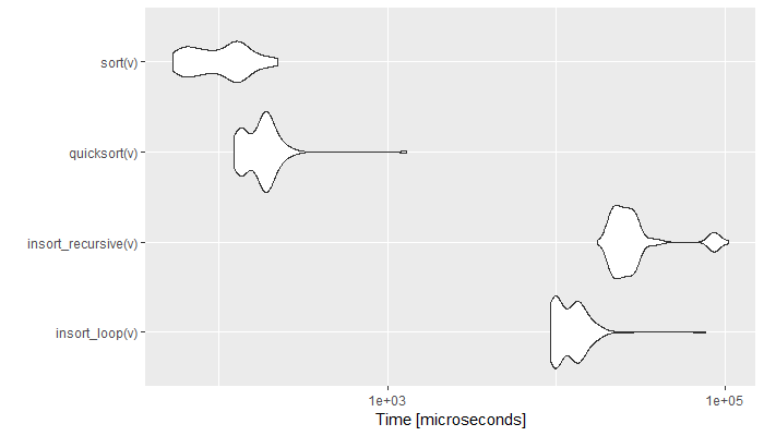

Figure 6.3: Comparison of Sort Speed (Time in log)

The graph shows the empirical time distribution of 100 runs of each function. As expected, the radix and quicksort algorithms perform a couple of order of magnitudes faster than the selection sorts. It is to be noted that the for loop implementation is generally faster than the recursive one.

6.2.2 Searching

Searching algorithms are a fundamental family of algorithms used whenever we need to recall the position of an element in an array. If numbers are stored in a random order in an array, then a linear search algorithm could be used to test for the presence of an element, where it simply loops through each element of the array and tests for equivalence against the search criteria, as shown in the following picture.

In code this translates to:

linear_loop <- function(v, x, i = 1) {
  while (v[i] != x) {
    i = i + 1
  }
  return(i)
}

This would perform in \(O\left(n\right)\) time in the worst case, given the element sought may be at the end of the \(n\) elements checked.

However, a binary search algorithm could be used instead were the data in the array to be sorted in an ascending (or descending) order. This algorithm, similarly to the quicksort in the previous section, is based on a divide and conquer logic. Here, the algorithm would pick the middle value of the array and test whether it is equal to the search criteria. If not, then the array is split in half, and the lower/upper section is fed back into the algorithm again depending on whether the search criteria is lower/higher than the middle value just tested, as in the following picture.

A code implementation of binary search algorithm is here provided in both its recursive and loop form.

# For loop implementation
binary_loop <- function(v, x, l = 1, h = length(v) - 1) {
  while (v[h + 1] != x) {
    n <- floor((h - l) / 2)
    l <- max(l, l + (n + 1) * sign(x - v[l + n]))
    h <- l + n - 1
  }
  return(h + 1)
}

# Recursive implementation
binary_recursive <- function(v, x, l = 1, h = length(v) - 1) {
  if (v[h + 1] == x)
    return(h + 1)
  else
  { n <- floor((h - l) / 2)
    l <- max(l, l + (n + 1) * sign(x - v[l + n]))
  return(binary_recursive(v, x, l, l + n - 1))}
}

Given this algorithm does not need to check against all \(n\) elements, it would be faster than the linear search approach as it would find the element in \(O\left(\log\left(n\right)\right)\) time.

In any algorithm considered so far, the distribution of the elements of the vector has not been considered. A possible variation on binary search consists in setting the midpoint interpolating between the position of our element between the extremes. In this case the midpoint would be calculated as:

\[\frac{S-V[1]}{V[n]-v[1]} \] where \(S\) is the value we are looking into a vector \(v\) of length \(n\). It is not difficult to refine our previous algorithm to include the new midpoint.

# For loop implementation
interpolation_loop <- function(v, x, l = 1, h = length(v)) {
  while (v[l] != x) {
    n <- ceiling((h - l) * (x - v[l]) / (v[h] - v[l] + 1))
    h <- max(sign(n) * h, l - 1)
    l <- l + n
  }
  return(l)
}

# Recursive implementation
interpolation_recursive <- function(v, x, l = 1, h = length(v)) {
  n <- ceiling((h - l) * (x - v[l]) / (v[h] - v[l] + 1))
  if (v[l] == x)
    return(l)
  else
    return(interpolation_recursive(v, x, l + n, max(sign(n) * h, l - 1)))
}

Given this algorithm starts from a midpoint which is close to its target value, it is significantly faster than the binary search approach as it would find the element in \(O\left(\log\left(\log\left(n\right)\right)\right)\) time.

However, the analysis above does not imply that one would always work with ordered data (even if that was the case in early statistical programming languages, such as SAS). In practice we do not only need to search for elements in unordered arrays, but we would find ourselves to search for strings and multiple values. Here is where hashing algorithms come in useful. Hashing is a different type of search technique, where elements in an array are assigned a key through an arithmetical function, known as hash function. A hash function creates a key value of the location of an element into a hash table, which is quicker to access than the original array. Hashing is the most common method of searching for strings and multiple values. In R hashing is implemented through its function match() which we have already encountered in other forms (%in%,Position and Find are all based on this function) in the previous chapters.

Here we present an empirical speed comparison with a randomly sampled ordered vector of 20000 elements.

library(microbenchmark)
library(ggplot2)

search_comparison <- microbenchmark(
    {v <- sort(sample(10^8, 20000, T)); x <- sample(v,1)}, 
    linear_loop(v,x), binary_loop(v,x),  binary_recursive(v,x), interpolation_loop(v,x), 
    interpolation_recursive(v,x), match(x,v), 
    times = 1000, control = list(order = 'inorder'))
autoplot(search_comparison[!grepl("sample",search_comparison$expr),])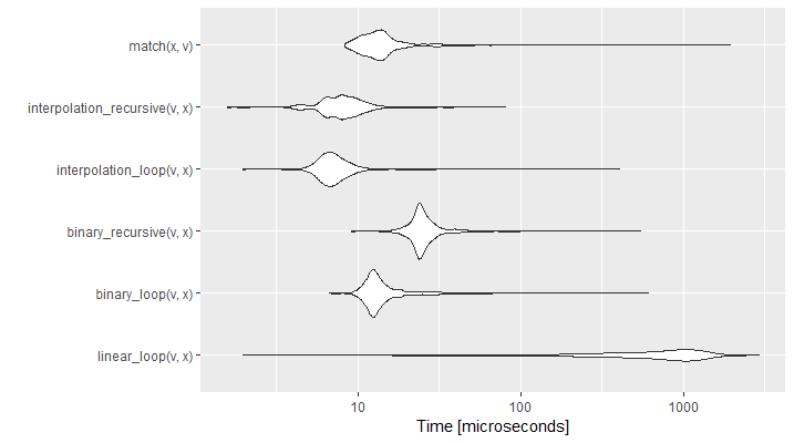

Figure 6.4: Comparison of Search Speed (Time in log)

The graph shows the empirical time distribution of 1000 runs of each function. As expected, the interpolation search is the fastest and linear search the slowest. Hashed search is not the most efficient, but it would significantly surpass the others if we had an unsorted vector. As previously, we noticed that the for loop implementation is generally faster than the recursive one. It is interesting to see that linear search, even if performing the worst overall, can result quicker in vectors where the element we are searching for is close to the head of the array.

6.2.3 Random Sampling and Monte Carlo

Random number generators (RNG) are a fundamental family of algorithms, used virtually in all actuarial simulations and also extensively used in cryptography. For our purpose we define a RNG as any algorithm that produces a sequence of random variables \(U_1; U_2\); with the property that each \(U_i\) is uniformly distributed between 0 and 1, and \(U_i\) are mutually independent.

Generating random numbers via an algorithm is usually preferred to using real random numbers because of speed of generation and easiness of replicating results. So called Pseudo Random Number Generators work by feeding a seed number into an algorithm. Each different seed can be used to produce a new dimension of random variates.

When measuring the effectiveness of a RNG, speed is not the only feature to look for. Other features include period, i.e. after how many numbers the series repeats, and discrepancy, i.e. how evenly spread are the random variates over the hypercube \([0,1]^d\). Algorithms with good discrepancy are of fundamental utility for Optimisation and Monte Carlo (MC) applications. As the reader already knows, MC is a method of simulation and integration, used for high-dimensional problems, ranging from physics to finance. Indeed, MC becomes increasingly attractive as the dimension increases, since its rate of convergence, \(O\left(n^{-1/2}\right)\) holds for all dimensions.

Different algorithms have been developed since the beginning of the last century, but most of them are built out of some simpler algorithms which are then combined to increase the randomness of the output. One of the most common are Linear Congruential Generators (LCG), i.e. recursive generators based on modulo operations. In formula: \[x_{i+1}=(ax_i+d)\mod m \hspace{3em} u_{i+1}=\frac{x_{i+1}}{m}\] where \(m\) and \(d\) are coprime, \(a-1\) is divisible by all prime factors of \(m\). A RNG which follows these properties would have a period of length \(m\).

It follows that for the simplest programming implementation we would choose an \(m\) multiple of 2, and an odd value of \(a\) and \(d\). We would use our seed to increase \(d\) and obtain new dimensions. This would be the recursive implementation of \(n\) points in \(seed\) dimensions.

LCG_RNG <- function(seed, n, m = 2 ^ 32, a = 8121, d = 1 + seed * 2) {
  if (n > 0) {
    d <- (a * d) %% m
    return(c(d / m, LCG_RNG(seed, n - 1, d = d)))
  }
}

The Mersenne Twister is another common RNG, used by R and Python as their default RNG. This algorithm is significantly more complex than the purpose of this book and features an impressive period of \(2^{19937} - 1\). Since in most programming languages the seed is set as global variable we define our Mersenne Twister function with an explicit argument for the seed.

Mersenne_Twister <- function(seed,n){
  set.seed(seed)
  runif(n)
}

For specific MC use a new family of RNGs has been introduced, so called quasi Random Number Generators (QRNG). Also known as Low-Discrepancy Sequences in mathematics, QRNGs consist of deterministic sequences which are typically highly predictable but more evenly distributed than other RNGs. qMC has a rate of convergence of \(O\left(n^{-1}log^dn\right)\) in dimension \(d\), if \(n\) is sufficiently large.

The Van der Corput sequence is the simplest Low Discrepancy sequence. It is obtained, given a base \(b\), by reversing the bits in the \(b\)-nary decimal representation of this naive sequence: \[\frac{1}{b},\frac{2}{b},...,\frac{b}{b},\frac{1}{b^2},\frac{b+1}{b^2},\frac{2b+1}{b^2},\frac{(b-1)b+1}{b^2},\frac{2}{b^2},\frac{2b+2}{b^2},...\]

An example is provided in the following figure.

Figure 6.5: Van der Corput Sequence

The easiest way to implement such a sequence in an algorithm is to use a recursive modulo operation to represent the \(b\)-ary representation of the naive sequence.

Van_der_Corput <- function(n, b, q = 0, f = 1) {
  while (n > 0) {
    f <-  f / b
    q <- q + (n %% b) * f
    n <- floor(n / b)
  }
  return(q)
}

Van der Corput sequences can be easily expanded in any dimension \(d\) by choosing two bases which are mutually coprime. Sequences which fulfil this condition are known as Halton sequences. Even though standard Halton sequences perform very well in low dimensions, correlation problems have been noted between sequences generated from higher close primes. To obviate this issue we will implement a lagged Halton sequence, which select Van der Corput sequences with prime bases at \(l\) distance.

Lagged_Halton_RNG <- function(b, n, l) {
  Vectorize(Van_der_Corput)(1:(l * n), b)[1 + 0:(n - 1) * l]
}

However since all bases needs to be coprime, to be able to simulate from this RNG we need a fast way to come up with a list of primes. Different algorithms have been developed to select all prime numbers smaller than \(n\). One of the simplest and most effective is Erathostenes Sieve. Erathostenes noticed that every non-prime number smaller than \(n\) needs to have at least a factor smaller or equal than \(\sqrt{n}\), hence it is possible to identify all prime numbers smallers than \(n\) by excluding the products of primes smaller than \(\sqrt{n}\). The algorithm is illustrated for \(n=120\) in the following figure.

Figure 6.6: Sieve of Eratosthenes

This sieve computes n primes in \(O\left(n\log\left(\log\left(n\right)\right)\right)\).

Eratosthenes_Sieve <- function(n) {
  n == 2 || all(n %% 2:ceiling(sqrt(n)) != 0)
}      
primes <- function(n) (1:n)[Vectorize(Eratosthenes_Sieve)(1:n)]

We finally have all the blocks to compare how different RNGs perform in a MC simulation exercise. We would try to calculate a simple integral, namely the ratio of the circle circumference to its diameter, also known as mathematical constant \(\pi\). A simple way of doing this is to simulate a bidimensional random series and count how many random variates lie inside or outside the unit circle, as shown in the following figure.

Figure 6.7: Pi Approximation, where the number of blue squares within the circle quarter divided by the total number of squares approaches pi/4 as n increases

We start by simulating 1000 random numbers for 51 dimensions using the three methods illustrated previously.

n <- 1000
set.seed(1)
x1 <- sapply(primes(233), Lagged_Halton_RNG, n, 409)
l <- ncol(x1)
x2 <- sapply(1:l, Mersenne_Twister, n)
x3 <- sapply(1:l, LCG_RNG, n)

We hence define our target function as the % MSE of our estimate per each \(n\) over the \(d\) dimensions and we plot the results for \(n=[100,1000]\) and for the three methods.

pi_MSE_percent <- function(n, x) {
  a <- sqrt(x[1:n, 1:50] ^ 2 + x[1:n, 2:51] ^ 2) <= 1
  mean((pi - colSums(a) * 4 / n) ^ 2) * 100
}

plot(100:n, sapply(100:n, pi_MSE_percent, x1), xlab = "n", ylab = "MSE %", main = "Pi approximation accuracy in log scale",type='l',log="y",las=1,ylim=c(0.02,2))
points(100:n, sapply(100:n, pi_MSE_percent, x2), col = 'red', type='l',log="y")
points(100:n, sapply(100:n, pi_MSE_percent, x3), col = 'blue', type='l',log="y")
legend('bottomleft', col = c(1:2,4), legend=c('Halton','Mersenne-Twister','Linear Congruential Generator'),lty=1)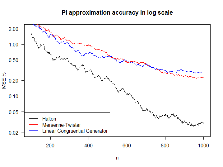

Figure 6.8: Comparison of RNG performance in MC

As expected the Halton sequence converges much faster than the other two, which have a similar performance. It is interesting to notice that, notwithstanding the complexity of Mersenne Twister, it does not differ significantly in performance compared to our simpler LCG.

6.3 Data structures

Arrays have already been discussed, but as aluded to above, they can host a variety of data structures:

• Ordered or unordered lists
• Queues (where data is stored in a First-In-First-Out basis)
• Stacks (where data is stored in a Last-In-First-Out basis, ie the “opposite” of a Queue)

Another common data structure is a tree, where parent nodes are assigned zero or more child nodes. This is akin to a non-linear version of an array, where each element can have more than one succeeding element. This data structure is useful for representing hierarchical relationships and file directories.

A graph however represents a more general network of nodes that are connected by edges. The edges can be directed (eg airplane flight paths) or undirected (eg friends in a social network). This complex data structure can be represented by simpler data structures in the form of an:

• Edge list, where connections between nodes are listed in an array
• Adjacency list, where a node is stored together with a list of all other nodes it is connected to, or
• Adjacency matrix, where for n nodes, an n x n matrix stores a binary value for each possible pairing.

As with the decision to use an ordered/unordered array above, the choice of which structure to implement is a function of the efficiency of the subsequent algorithms required and their likely usage. The intrinsic relationship between algorithms and data structures can also be demonstrated. A breadth-first search algorithm would explore a graph using a queue as an internal memory store of nodes not yet explored, whilst a depth-first search algorithm would explore a graph using a stack as an internal memory store, prioritising exploring the depths of a given branch before moving onto another.