2 Environment set up

This section describes the tools typically used in creating a programming solution, along with their key features.

2.1 Notepad

In its essence, code is simply a plain text file that is written using a certain language convention. For example, typing the following characters into Notepad would create an R function that returns the factorial of a given number n.

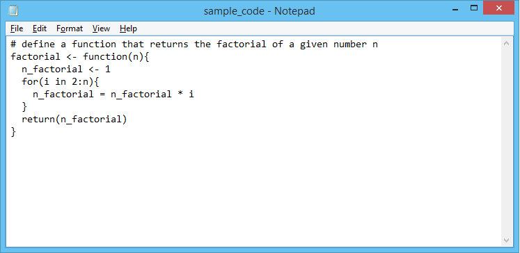
$\label{fig:figs}Using Notepad for coding a function in R$

Figure 2.1: Using Notepad for coding a function in R

The power of Notepad cannot be understated; entire websites can be created using Notepad alone. However, this is like saying an entire book can be written with pen and paper alone. Whilst technically true, other tools exist that make the job much easier and faster.

2.2 Text editors

Other text editors have additional features when compared to Notepad and are suited to writing code. The choice of text editor is largely subjective and dependent on the person, the coding challenge and language. A lot of popular text editors are available for free, for example:

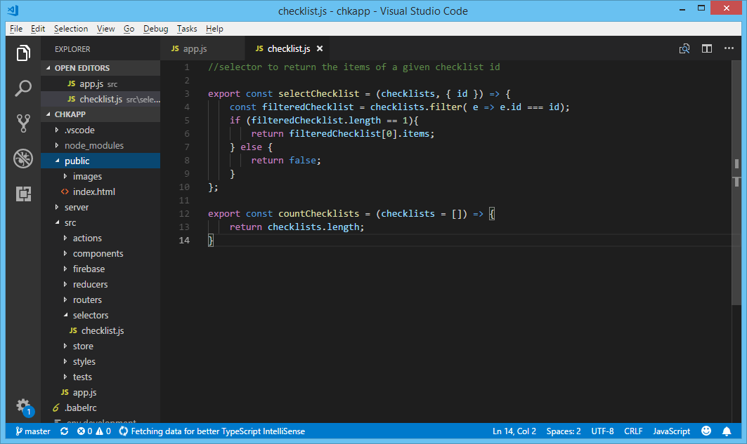
$\label{fig:figs}A node.js project in Visual Studio Code editor$

Figure 2.2: A node.js project in Visual Studio Code editor

Note that Microsoft Word is not a plain text editor, it is a word processor. Text entered in Word is rich text, embedded with metadata about formatting, borders etc. Microsoft Word is not used for coding.

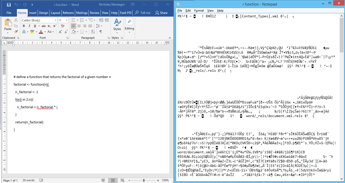
$\label{fig:figs}A Microsoft Word file, r function.docx, as seen by Notepad$

Figure 2.3: A Microsoft Word file, r function.docx, as seen by Notepad

The features of each editor are different. Using Notepad++ as an example, the basic features in a good text editor are now discussed.

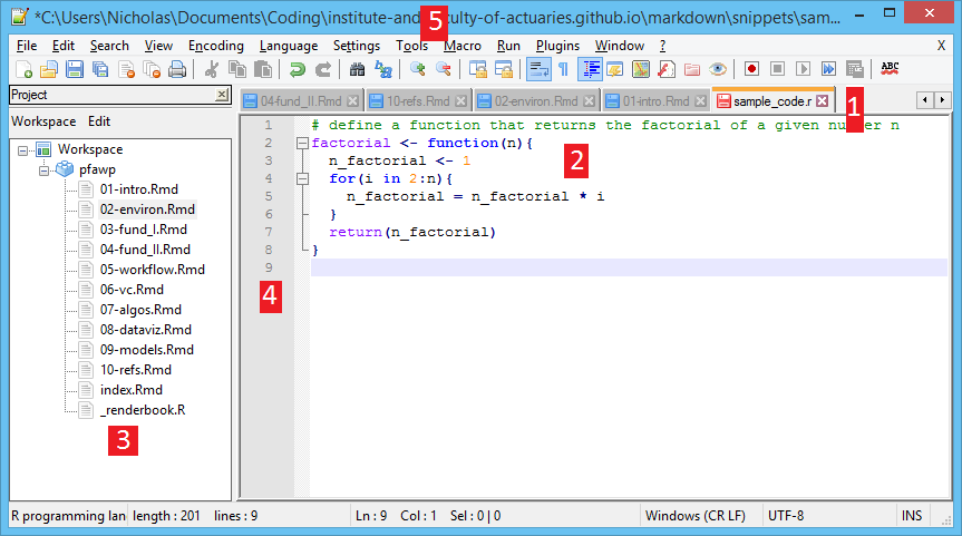
$\label{fig:figs}Using the Notepad++ text editor$

Figure 2.4: Using the Notepad++ text editor

2.2.1 Tabbed browsing

Several files can be open at the same time in different tabs, as shown by 1 in Figure 2.4. Given a structured coding solution may span several files, this feature is useful for quickly switching between files. The project pane, 3 in Figure 2.4, also supports quick file switching (where files can also be created, deleted or renamed).

The tab can also indicate whether the file has unsaved changes in it (here shown as a red icon, relative to the blue icon tabs that contain no unsaved changes).

2.2.2 Interactive code input

Whilst Notepad merely showed black text on a white background, text editors implement syntax highlighting, as seen at 2 in Figure 2.4. Special words, variable types and symbols are given different colours, to enable better understanding.

The editor can also have autocompletion, where words are suggested as you type, to speed up typing speed and accuracy. In the example beneath, after defining the function factorial, just typing the letters fa on line 9 is enough to prompt the editor to suggest factorial as an input.

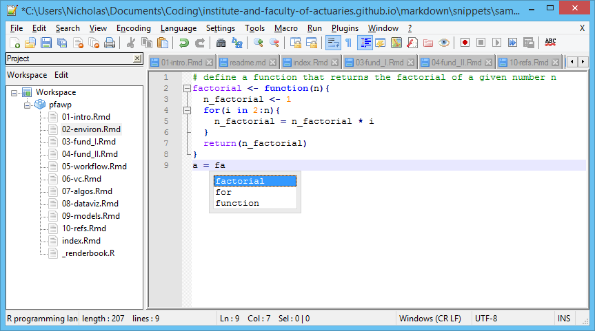
$\label{fig:figs}Autocomplete suggests words based on the code so far$

Figure 2.5: Autocomplete suggests words based on the code so far

Editors can also show the corresponding closing/opening bracket for a selected bracket. By placing the cursor next to the bracket on line 6, the neighbouring bracket turns red, as does its pair up on line 4.

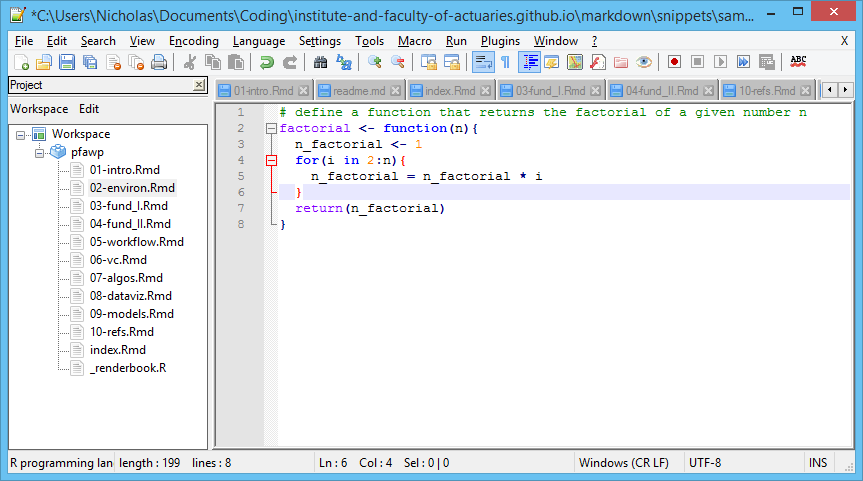
$\label{fig:figs}Matching brackets highlighted in red font$

Figure 2.6: Matching brackets highlighted in red font

Other highlighting features include highlighting all other instances of a selected word, quick variable renaming and more.

2.2.3 Code mapping

Next to the coding pane, 4 in Figure 2.4 details some meta data about the code. Principally, line numbering can be seen here. In addition, subsections of the code (like function definitions, loops) can be highlighted and even collapsed to hide (but not remove) lines to get a higher level view.

Some editors allow code to be debugged and this is where breakpoints would be placed.

2.2.4 Additional tools

In the menu bar, 5 in Figure 2.4, additional code writting features can be found. Macros are a useful tool - keystrokes can be recorded, saved, and repeated throughout the file. This is handy for reformatting code into a new structure, or for tidying data. Plugins are external add-ons to the text editor that can bring further functionality.

Editors can also allow for further customisation, like changing its appearance.

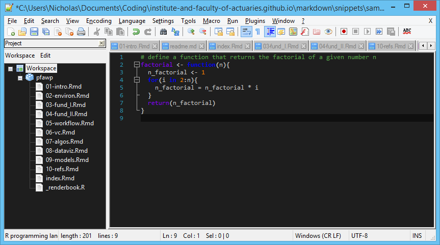
$\label{fig:figs}Notepad++ with a custom dark theme$

Figure 2.7: Notepad++ with a custom dark theme

2.3 Running Code

Once the code is written, it needs to be run. Typically programmers will be coding source code in a high level programming language, like R. This will need to be converted into machine code to enable the computer to run it. Depending on the language used, either a compiler performs this translation to create an executible file that is executed later, or an interpreter converts and executes the code as it is read in. Discussion of compliled vs interepreted code is outside the scope of this book.

The interpreter for R can be downloaded from https://www.r-project.org/ and run either in the command line or via an IDE.

Alternatively, code can be run online using platforms such as repl.it.

2.4 Integrated Development Environment (IDE)

IDEs add additional features to text editors enabling the coder to not only edit the code files, but run them too. Again, there are several popular packages available. Whilst text editors can support most, if not all, coding languages (as they are only editting plain text files), IDEs tend to target a subset of languages so the choice of IDE is driven more by the language chosen than its features.

Net Beans
Eclipse
Visual Studio
RStudio
Microsoft Office has a VBA IDE as standard, eg hit Alt + F11 in Excel

For the purposes of this guide, the aspects of an IDE will be explained using RStudio.

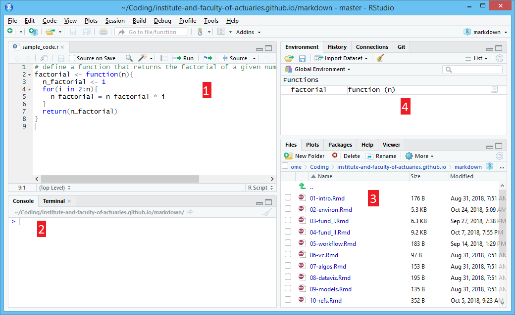
$\label{fig:figs}RStudio is a popular IDE for R$

Figure 2.8: RStudio is a popular IDE for R

2.4.1 Text Editor

IDEs themselves normally contain a text editor, as seen at 1 in 2.8. This will probably contain fewer features than a stand alone text editor, although a lot of the essential features should be available.

2.4.2 Console

The main IDE feature is the console, as seen at 2 in 2.8. Individual lines of code can be entered and run here, and the console will return the statement’s output. Entire files and programs can be run from here too, and examined in real time for the purposes of debugging code (discussed later).

2.4.3 Project Pane

As with text editors, a project workspace can be viewed at 3 in 2.8. RStudio also has other views that can be seen here, such as a list of the packages available, plot outputs and the contents of help files.

2.4.4 Environment

Given an IDE can run code in real time, the environment pane at 4 in 2.8 can be used to examine variables and their values. For example, Figure 2.8 has the function factorial already defined (as per the code in the text editor) and we can click into this here when debugging.

2.4.5 Debugging

One of the main uses of an IDE is to debug code. If we were to debug the factorial function, we could place a breakpoint on one of the lines in the function defintion by clicking next to the relevant line number.

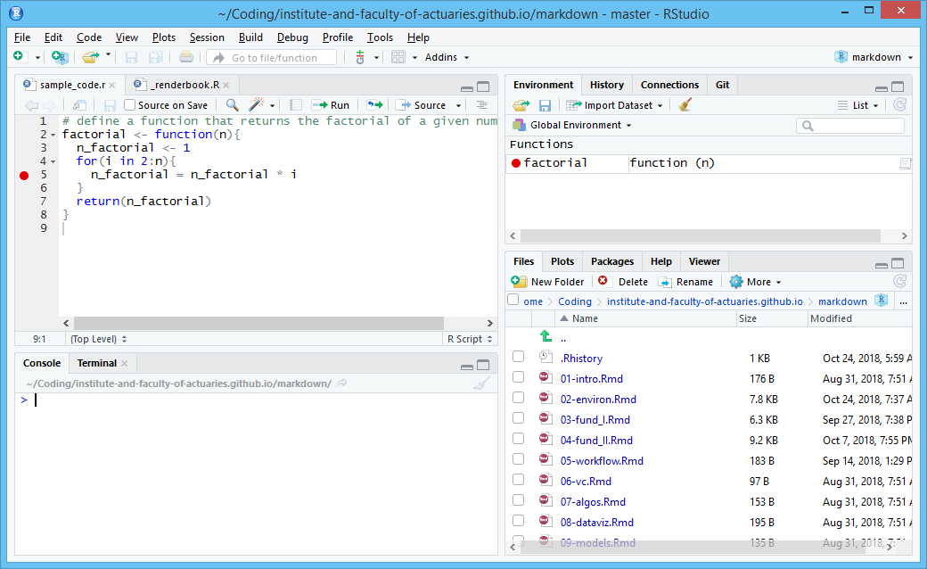
$\label{fig:figs}RStudio with a breakpoint on line 5$

Figure 2.9: RStudio with a breakpoint on line 5

Now, if we were to run the function in the console by entering factorial(4), we can inspect the function and its variables during its operation.

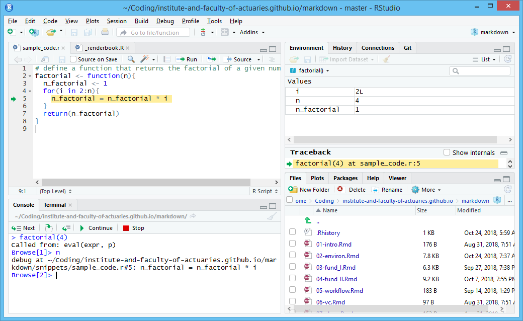
$\label{fig:figs}RStudio paused at line 5$

Figure 2.10: RStudio paused at line 5

In the environment pane, we can see the function variables n_factorial, n and i are now displayed, together with their values. We can now step through the code to see how these values change with time, and check whether that progression is inline with what is expected of it. The text editor pane illustrates our position in the code (with a green arrow) as we progress.

2.5 Notebooks

When conducting analytics using code it is becoming increasingly popular to use a notebook file format. This makes it easy to combine text, code and analysis output (e.g. tables or charts) in the same document. When a notebook file is run, the code within is executed and the analysis results are inserted automatically into the document, which can then be converted to html, pdf or MS Word format for publication. These formats improve the reproducibility of the analysis and avoid the need to copy-paste results into final documents or presentations.

Two popular formats are R markdown used to create this book (and popular with those using R and RStudio) and Jupyter notebooks (popular for Python but supporting over 40 lanuages). Note that, despite the name, R Markdown supports several languages.

In R Markdown descriptive text can be mixed with code for output in a range of publication formats.

```{r chunk-label, echo = FALSE, fig.cap = 'A figure caption.'}
1 + 1
rnorm(10)  # 10 random numbers
plot(dist ~ speed, cars)  # a scatterplot
```