Introduction
This analysis compares the predictive power of a Feed-Forward Neural Network and a Gradient Boosting Machine against the industry-standard Chain Ladder model. The core of this work is to showcase how these modern algorithms can offer improvements in performance and to provide a clear understanding of their mechanics, thereby encouraging their wider adoption in actuarial science.
This work is based on the Neural Network and GBM models as set out in our previous blog by Jacky Poon, with sincere appreciation to Nigel Carpenter for reviewing this post.
The code for this analysis is available in the Jupyter Notebook and can be run in a local environment or on Google Colab. The notebook contains all the necessary steps to replicate the results, including data preprocessing, model training, and evaluation.
Summary of Findings
The empirical results of this comparative study indicate that the Feed-Forward Neural Network (FFNN) and the Gradient Boosting Machine (GBM) outperform the traditional Chain Ladder (CL) method. This superiority is particularly evident in higher, more recent, occurrence periods, where the CL method suffers from increased estimation error due to the inherent scarcity of mature data.
Specifically, the Feed-Forward Neural Network achieves better performance than the Gradient Boosting Machine, yielding smoother predictions, whereas the GBM output is more discontinuous due to its stepwise optimization.
Throughout the exercise, both algorithms were tested using various preprocessing techniques to explore how data structures influence their behavior. These tests revealed that data preparation significantly affects each model’s performance in distinct ways, reflecting their underlying learning mechanisms.
The Dataset
The dataset used is SPLICE (Synthetic Paid Loss and Incurred Cost Experience), which is based on the R data simulation package SynthETIC (Synthetic). An introduction to the package can be found here (SynthETIC intro).
The analysis is conducted using the Splice 5 dataset, which is specifically characterized by long-tailed claims and highly volatile development patterns. Unlike simpler datasets, this version provides a more granular view of the claims process, featuring a dedicated record for every transaction across each development period. This level of detail, combined with the inherent instability of the claims’ evolution, presents a challenging benchmark for testing the predictive capabilities of both the FFNN and the GBM.
In terms of feature richness, the SPLICE dataset is relatively parsimonious, relying primarily on a combination of temporal indicators and monetary amounts. The input space is essentially defined by date-based features and historical payment information, requiring the models to extract meaningful patterns from a limited set of predictors. The table below provides a detailed breakdown of the variables utilized in the final model training:
Variables
| Variables included | Description |
|---|---|
| notidel | Reporting delay from occurrence |
| occurrence_time | Time of accident |
| development_period | Time of payment from occurrence |
| payment_period | Absolute time period of the transaction |
| has_payment_to_prior_period | Binary indicator of payments made prior to the current period |
| log1_payment_to_prior_period | Natural logarithm of (1 + cumulative payments) up to the prior period |
| payment_count_to_prior_period | Total count of payment transactions up to the prior period |
| transaction_count_to_prior_period | Total count of all transactions up to the prior period |
While features related to outstanding claims were initially considered, they were ultimately excluded to maintain consistency with previous analyses in this series. The underlying rationale is that outstanding-based features are heavily influenced by a company’s specific claims-handling procedures and internal valuation policies. Including them could yield results that are difficult to generalize or potentially inconsistent when applied to different real-world operational frameworks.
Test/Train Splits
| A fundamental challenge in actuarial modeling is ensuring that a model’s predictive power is evaluated under conditions that mimic real-world forecasting. Unlike standard machine learning tasks where data points are often treated as independent, insurance claims development is inherently chronological. To maintain the integrity of this exercise, our splitting strategy focuses on the following pillars: |
Time-based Cutoff The primary objective of this split is to prevent “look-ahead bias” — the accidental use of future information to predict past events. By partitioning the data based on the payment_period, we simulate a true valuation date. All transactions occurring after this cutoff are withheld during the training phase, forcing the models to project future developments using only the information that would have been available to an actuary at that specific point in time. |
Rolling Origin Cross-validation To improve our trained models effectiveness at predicting future time periods we implemented a rolling origin cross-validation strategy via a custom RollinOriginSplit function. This function partitions the data into train and evaluation folds where the train partition data will always be from time periods that precede the evaluation data. This ensures we assess the training performance of the FFNN and GBM across future temporal segments, thereby selecting hyperparameters that are tuned for generalizability across future time periods rather than simply optimizing for historic trends. |
| The following table summarizes the implementation details of these methods: |
| Split Method | Description |
|---|---|
| Time-based Cutoff | Data is partitioned based on the payment_period. Transactions up to the cutoff are used for training. |
| Cross-validation | A RollingOriginSplit function is defined and used for cross validation in model training. |
Data Augmentation Strategy - Backdating
Traditional reserving approaches typically involve a recursive prediction loop. This arises because in the training data the response at time t is structured to be a function of variates up to time t-1, ie it is a one-step ahead prediction process.
We make use of backdating, an approach that augments the training and test data so that the resulting model can predict ahead across the full range of steps required. The model can be trained in a single training pass and the predictions made for all future steps in a single prediction pass. This approach was first introduced in the paper by Maximilien Baudry “Non-parametric individual claim reserving in insurance” which we covered in our 2020 blog post series. Our implementation of backdating is an enhanced version developed by Jacky Poon and used in our 2023 blog post.
Generating Historical Snapshots
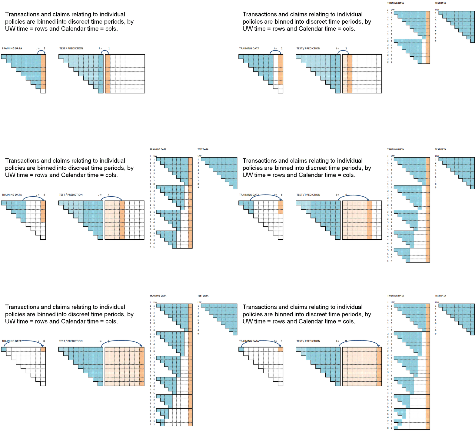
- Backdating consists of generating multiple versions of the historic claim training data, each simulating a different historical “as-of” date. By providing these varied temporal snapshots, we enable the model to predict forward across the full range of future steps.
- Temporal Shifting: The
development_periodis adjusted by thebackdate_periodsfactor, effectively “sliding” the claim’s history to create new training samples. - Data Enrichment: This allows the model to “see” the same claim at different stages of its life cycle, significantly increasing the diversity of the training signals.
The backdating approach is illustrated in an animation taken from the notebook referenced in our 2020 blog post
| Augmentation Feature | Description |
|---|---|
| backdate_periods | Number of periods to shift back the “as-at” date for simulation. |
| data_as_at_dev_period | Adjusted development period used as the model’s reference point. |
| payment_period_as_at | Original payment period, preserved to link back to actual transaction time. |
Dataset Construction and Sampling
While backdating simplifies the training and prediction process it introduces a bias in the training data which, due to backdating augmentation, will contain more observations from older occurrence periods. It also significantly increases the volume of training data which can adversely affect model training times. To handle the increase in data volumes and the bias to older occurrence periods, we have used a dynamic sampling strategy during training instead of feeding the full dataset in all at once.
We implemented this dynamic logic through a custom function called claim_sampler, which introduces a stochastic element into the FFNN model workflow. For any given epoch or batch, it samples a single historical snapshot for each unique (claim_no, development_period) pair. This both reduces the size of the training dataset and reduces the bias from older occurrence periods. We used this logic exclusively for the Neural Network when training on the nn_train_full dataset, giving the model a fresh “perspective” on each claim’s history with every pass. This sampling approach doesn’t fit with the Gradient Boosting workflow, so we achieved a similar effect for the GBM using a weighting scheme. That way, despite their structural differences, both models digest an equivalent distribution of information, keeping our benchmark comparison fair and rigorous.
This setup continually exposes the model to varied temporal angles across epochs, making it much better at generalizing from incomplete data. At the same time, dynamic sampling keeps computational costs down and stops the model from overfitting to static snapshots while still squeezing value out of the full augmented dataset.
To benchmark how data layout influences overall performance, we built a control dataset (nn_train) that skips dynamic sampling entirely. Instead, it relies on a representative sampling method, picking exactly one record per claim_no and development_period pair. This delivers a clean, balanced look across the entire claim lifecycle, letting us test how both models adapt to a traditional static dataset versus a more dynamic setup.
Finally, we added a dedicated feature for “backdated” periods to help the algorithms separate and process historical records correctly. Giving the models this explicit temporal context ensures they accurately map the timeline between transaction dates and the original claim events.
Models
In this study, we evaluate and compare different modeling architectures to project claim payments. The primary focus is on a customized Feed-Forward Neural Network (FFNN) designed to handle the specific distribution of insurance losses and the “long-tail” nature of the SPLICE 5 dataset.
Feed-Forward Neural Network (FFNN)
The FFNN is implemented as a regression model with a single hidden layer, specifically tuned to emulate the behavior of a Generalized Linear Model (GLM) with a log-link function, while allowing for non-linear interactions through its architecture.
Architecture & Hyperparameters
To build an effective predictive engine, we must consider how the data is transformed at each stage of the network. The process begins at the Input Layer, where we address the model’s sensitivity to data magnitudes. By applying a MinMaxScaler, we normalize all features into a [0, 1] range; this ensures that no single variable dominates the learning process simply because of its scale, allowing for more stable and uniform gradient updates.
Once the data is normalized, it passes into the Hidden Layer. This is the core of the architecture where the “learning” of non-linear patterns happens. By employing a dense layer with a ReLU activation, the network is able to identify complex interactions between the claim features—such as the relationship between reporting delays and payment volatility—that traditional linear frameworks might overlook. To ensure that this learning remains robust, we integrate Regularization techniques like Dropout and Batch Normalization, which stabilize the optimization landscape and prevent the model from overfitting on noisy insurance data.
We have utilized a Poisson Loss function in the model training process. A Tweedie Loss function would better reflect the distribution of the underlying training data, however the tweedie loss is not natively available in the scikit-learn python packages commonly used to train the neural networks and would require a custom loss function to be written. We use a log link function so that the model predicts the logarithm of the target variable, useful for such a skewed distribution as this where there are a lot of small claims, and far fewer very large claims. This means that later on we use an exponential function \(Y = \exp(XB)\) to convert the values back to normal claim sizes, this process means predictions are strictly non-negative.
Finally, the Output Layer starts from a controlled baseline, using weights initialized to zero and a pre-calculated bias to ensure rapid and stable convergence.
The following table summarizes the implementation details of this architecture:
| Component | Description |
|---|---|
| Input Layer | Feature scaling via MinMaxScaler [0, 1]. |
| Hidden Layer | Single dense layer with ReLU activation. |
| Loss Function | Poisson Loss, selected as best alternative in absence of the availability of tweedie loss. |
| Regularization | Dropout and Batch Normalization for stability. |
| Output Layer | Linear layer with zero-weights and init_bias. |
| Output Activation | Exponential (Log Link). |
Hyperparameter Tuning Space
Finding the optimal balance between model complexity and generalization requires a systematic search through the hyperparameter space. For this purpose, we utilized a RandomizedSearchCV approach. Unlike a traditional Grid Search, which exhaustively tests every possible combination, Randomized Search samples a fixed number of configurations from specified distributions. This is often more efficient, as it allows for a broader exploration of the parameter space within a reasonable computational timeframe, focusing on the variables that most significantly impact model performance.
Crucially, this search was guided by a Rolling Origin Split (5 folds). By using a walk-forward validation strategy, we ensured that the selected hyperparameters were robust across different time horizons, effectively mimicking how an actuary would update the model as new calendar periods emerge. The following table details the search space explored:
| Parameter | Search Space / Range |
|---|---|
| n_hidden | [5, 10, 20] nodes |
| Dropout rate | [0, 0.25, 0.5] |
| L1 Penalty | [0.0, 0.001, 0.01, 0.1] |
| Weight Decay (L2) | [0.0, 0.001, 0.01, 0.1] |
| Max Learning Rate | 0.05 |
In practical application you may wish to search a wider range of values in each parameter as well as a wider range of parameters. This will slow down the model training in which case it may be helpful to use a HalvingRandomSearchCV approach.
Refitting Logic
Once the best parameters from the selected searched space are identified, the model is refit using the full training pool with the following enhancements:
- Dynamic Resampling: The
claim_sampleris triggered every few iterations (rebatch_every_iter) to expose the model to different “backdated” snapshots of the same claim. - Feature Preservation: The
ColumnKeeperensures only the relevant features (including thebackdate_periodsindicator) are fed into the network. - Rolling Origin CV: Validation is performed on chronological “future” periods, ensuring the model’s predictive power is tested in a realistic reserving scenario.
This model has been tested using different training data sets, but the best performance was achieved using the nn_train_full dataset with the sampling techniques previously mentioned.
Gradient Boosting Machine (GBM)
As a benchmark for the neural network, we implemented a Gradient Boosting Regressor. This model is particularly effective at capturing complex, non-linear relationships and interactions without requiring the extensive feature scaling (like normalization) needed by deep learning architectures.
The core logic of a GBM lies in its ensemble nature: it builds a series of decision trees sequentially rather than in isolation. Each new tree is designed to predict the “residuals”—or the errors—left behind by the previous ones. By moving in the direction that minimizes the loss function, the model iteratively refines its estimates. Using a histogram-based approach further optimizes this by binning continuous features into discrete intervals, which significantly accelerates the training process and reduces memory usage without sacrificing accuracy.
Model Configuration
In order to provide a meaningful benchmark the configuration of the Gradient Boosting Machine was setup to be consistent with the Neural Network architecture, particularly regarding the underlying distribution of the target variable. So the GBM also uses an exponential link function and a Poisson Loss function, even though tweedie loss is natively available for the scikit-learn GBM.
This choice mirrors the log link and the loss function used in the FFNN, allowing both models to operate under the same assumption: that claim payments are strictly non-negative and follow a distribution where the variance is proportional to the mean. By synchronizing the loss function across both architectures, we create a more controlled benchmark, ensuring that any performance differences arise from the models’ structural abilities to capture patterns rather than from differing statistical objectives.
The following table summarizes the core components of the GBM configuration:
| Component | Description |
|---|---|
| Model Type | HistGradientBoostingRegressor, chosen for its efficiency in handling large datasets through feature binning. |
| Loss Function | Poisson Loss, selected for consistency with the the FFNN constrained approach. |
| Feature Selection | Managed via ColumnKeeper to ensure strict consistency with the FFNN feature set. |
Hyperparameter Tuning Space
Similarly to the FFNN, we tuned the GBM using a RandomizedSearchCV with a Rolling Origin Split (5 folds) to identify the optimal configuration. The tuning process specifically focuses on controlling the model’s complexity to avoid overfitting.
A key parameter in this search is L2 Regularization, which adds a penalty proportional to the square of the weights (or leaf values) to the loss function. In the context of Gradient Boosting, this “shrinks” the influence of individual trees, preventing the model from becoming overly sensitive to specific noise in the training data and ensuring more stable, conservative predictions across the claims’ development.
| Parameter | Search Space / Range |
|---|---|
| max_iter | [500, 1000, 2000, 5000] (Number of boosting rounds) |
| learning_rate | [0.03, 0.07, 0.1] |
| l2_regularization | [0, 0.001, 0.01, 0.1, 0.3] |
| Validation | Rolling Origin Split (5 folds) based on payment_period. |
Key Differences in Strategy
The most significant distinction between the two approaches lies in their approach to mitigating data bias arising from backdating. While the FFNN leverages a dynamic sampler to observe diverse “perspectives” of the claims’ history in each iteration, this cannot be used in the GBM algorithm. Instead our tests revealed that the GBM can achieve comparable results when trained on a backdated dataset, provided a weighting approach is implemented.
We conducted extensive sensitivity analyses across various data structures and preprocessing techniques to evaluate how each algorithm adapts to different levels of granularity and sampling frequencies. These tests revealed that the GBM’s learning mechanism becomes most effective when processing the full historical trajectory, as long as we assign weights—specifically \(1/n\) for repeated claim numbers to reduce the disproportionate influence of long duration claims. By tailoring the data input to these specific strengths, we ensure that the subsequent comparison reflects both models in their most effective operational states, providing a more rigorous assessment of their true predictive potential.
# Findings
In this section, we evaluate and compare the out-of-sample performance of our two primary architectures. Having identified the optimal training strategies for both—leveraging dynamic sampling for the FFNN and a weighted augmented structure for the GBM—we now test their predictive power on the SPLICE 5 test set using a realistic temporal split.
Comparative Model Performance
We compare the ultimate estimates produced by the FFNN and the optimized GBM against the traditional Chain Ladder method. The performance is evaluated by measuring the deviation from the True Ultimate values across all occurrence periods. We tested different seeds in order to asses the impact of the algorithms’ volatility.
Average Error Metrics
The following table summarizes the Average Error Percentage (AV Error%) across the entire development history using 5 different seeds. This metric provides a high-level view of model reliability, measured as the deviation of the total estimated reserve (Ultimate) from the actual value at claim closure.
| Seed | Chain Ladder | FFNN | GBM |
|---|---|---|---|
| N1 | 16.70% | 8.31% | 9.88% |
| N2 | 16.70% | 7.90% | 10.16% |
| N3 | 16.70% | 10.79% | 10.13% |
| N4 | 16.70% | 12.76% | 14.12% |
| N5 | 16.70% | 9.94% | 15.46% |
Both FFNN and GBM outperform the traditional Chain Ladder—which obviously always produces the same results because it is deterministic—effectively reducing the average error by a substantial margin. While the FFNN achieves the lowest average absolute percentage error, the GBM also demonstrates competitive performance, especially considering its different structural approach to the data.
The results have been run across a range of seed values and produce consistent results, showing that while deep learning and tree-based models use different internal logic, they both reach a superior level of precision compared to legacy methods when supported by specialized data augmentation and a robust weighting strategy.
Analysis of Ultimate Projections
The following visualizations illustrate how each model tracks the “True Ultimate” values across different occurrence periods, these findings are related to the first seed.
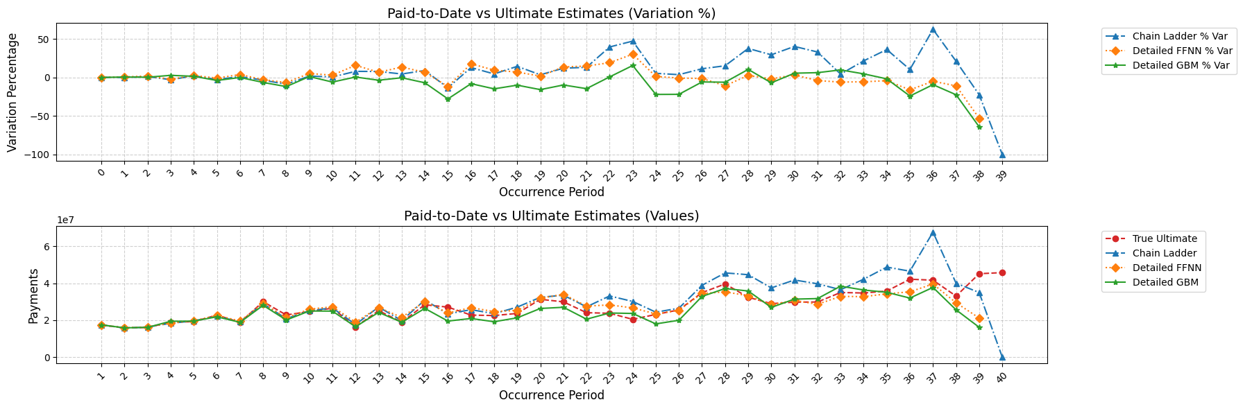
This visualization clarifies the operational strengths of each approach. Looking at the Variation % plot, the Chain Ladder (blue line) exhibits more volatility in recent occurrence periods (30–40), swinging from overestimation peaks exceeding 50% to a total collapse in the final period. This highlights the method’s failure when faced with sparse recent data.
In stark contrast, both GBM and FFNN remain remarkably anchored. Even in the “tail” periods where available data is minimal:
FFNN (Orange): Achieves the highest performance, with a path that remains almost indistinguishable from the True Ultimate throughout the claim history. Its ability to maintain stability without losing accuracy makes it the most reliable model in this comparison. The FFNN architecture allows it to capture the changes in claim development in the Splice 5 dataset more effectively, providing the most accurate projections even in the most recent time periods where the risk of mis-reserving is highest.
GBM (Green): While highly stable and free of erratic spikes, the GBM shows a consistent tendency toward underestimation at the portfolio level, particularly in recent periods.
The core takeaway is that traditional methods reach a clear breaking point in complex scenarios. The Chain Ladder loses its predictive power in recent periods, where its lack of structural complexity leads to volatile estimates. In contrast, our data-driven approach for the “tail” appears to function better than the CL logic, providing a more grounded extrapolation.
AvE Plot
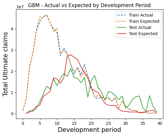
In the following plots, we show the training and test set performance of the two models, considering the first seed only for simplicity.
| FFNN | GBM | |
|---|---|---|
| Development Period | 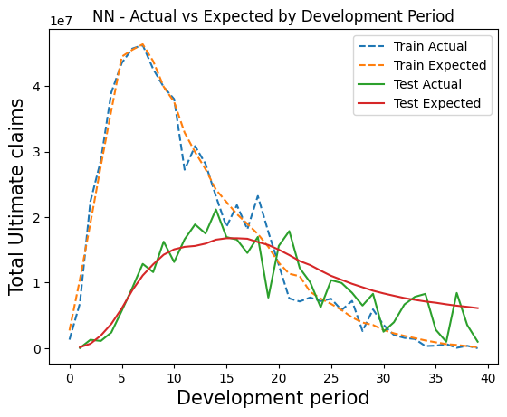 |
 |
| Occurrence Period | 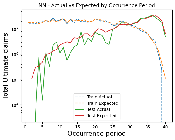 |
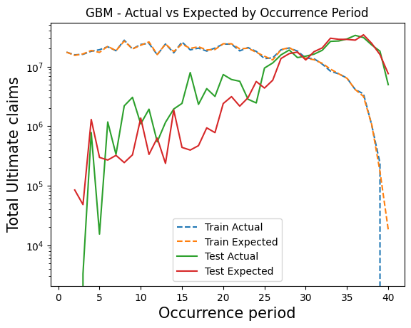 |
These plots show how the GBM tends to overfit during training and to be more volatile on the test set, while the FFNN produces smoother results because of its flexibility and ability to approximate continuous functions.
Granular Performance: RMSE Analysis
While looking at ultimate estimates provides one view of overall accuracy, analyzing the Root Mean Square Error (RMSE) on incremental payments can provide insight on the relative variance in predictions from different models. We use the RMSE for ease of calculation and understanding but acknowledge that in practice it would be better to use a metric that is consistent with the loss function used in model training. In our case that would ideally be a tweedie deviance measure were it not for the fact that we had to resort to poisson loss due to restrictions in the scikit learn package!
The Granular Paradox: Overall Error Summary
The following table presents the total RMSE calculated across all individual predictions in the test set using five different seeds.
| Seed | Detailed FFNN | Detailed GBM |
|---|---|---|
| N1 | 54,913 | 57,253 |
| N2 | 55,074 | 57,013 |
| N3 | 55,406 | 57,577 |
| N4 | 55,676 | 57,003 |
| N5 | 54,960 | 56,429 |
The FFNN can be seen to outperform the GBM for all the seeds, though the magnitudes of the differences are not so great. The volatility between the different trials is very small, this makes sense considering that these models are optimized in order to minimize an individual loss functions, not a portfolio measure like AV%. Usually, what happens, is that the optimal solution at individual level could cause some delta at portfolio level because of the sum of a lot of very small errors on individual records.
Error Distribution over Time
We decompose the RMSE by Occurrence Period and Development Period on seed one, this reveals where the models truly diverge.
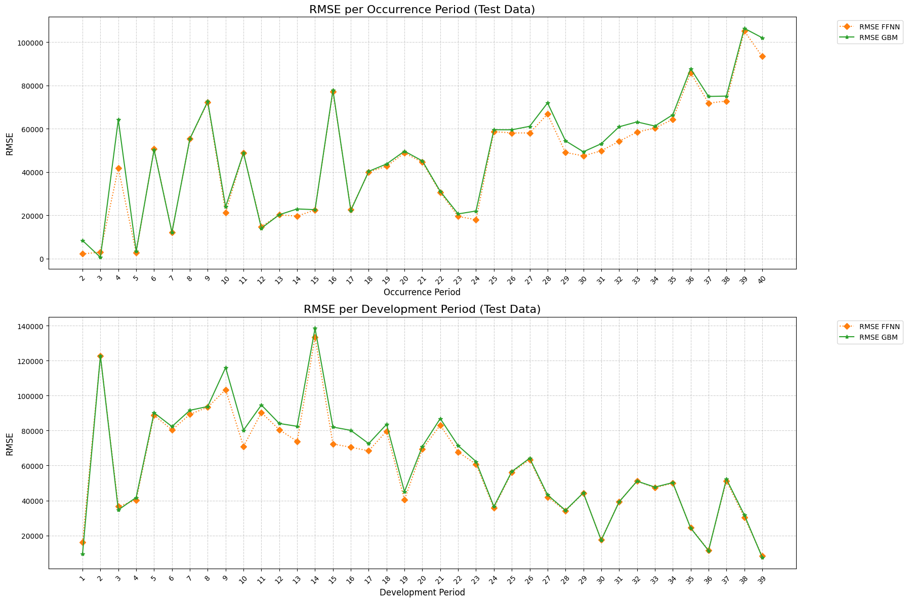
In both plots, the performance trajectory is highly synchronized across the entire timeline. While the FFNN shows lower RMSE in basically all the periods.
Analysis of Test Dataset: Quantile-based AvE Plots
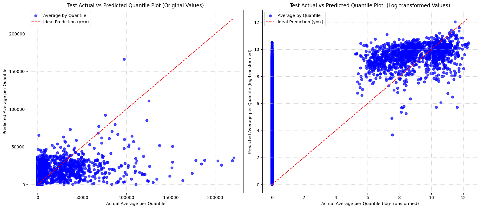
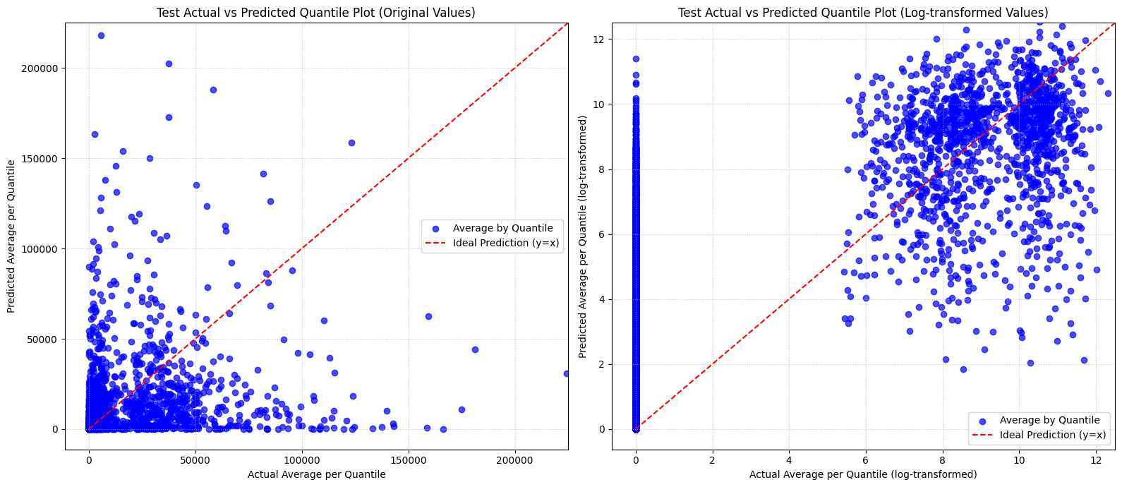
To evaluate the fit quality across the entire distribution, we utilize Quantile-based Actual vs. Expected (AvE) plots. In these charts, the test observations are grouped into 5,000 quantiles based on their predicted values; for each quantile, the average predicted value is plotted against the average actual outcome. The ideal calibration lies on the red dashed line (\(y = x\)). Points falling below the line indicate a model underestimation, while points above indicate an overestimation. By analyzing these relationships on both original and logarithmic scales, we can assess how well the models capture the central tendency and the extreme values of the distribution.
Neural Network (FFNN)
The FFNN demonstrates a good overall calibration for small-to-mid-sized claims, with predictions generally well-centered along the \(y=x\) reference line. However, clear limits emerge at the extremes: on the original scale, the model systematically underestimates large claims, while the log-transformed plot confirms a persistent struggle with zero-payment outcomes at \(Actual = 0\).
Gradient Boosting Machine (GBM)
Similarly, the optimized GBM captures the central trend for standard claims, but exhibits higher dispersion than the FFNN. On the original scale, its predictions are far more volatile, showing severe overestimation outliers alongside the systematic underprediction of large losses. In the log plot, it mirrors the FFNN’s structural inability to output exact zero payments
Interpretation and Actuarial Observations
Comparing both architectures across the test dataset reveals clear empirical trends in how each model handles different claim sizes and volatility levels.
The “Zero-Payment” Challenge
The log-transformed plots highlight a shared structural limitation: the handling of zero-payment outcomes. Both models display a dense vertical column at \(Actual = 0\), confirming an inability to output exact zeros.
Instead of capturing data sparsity, both architectures assign small positive expected values to inactive claims. This occurs as a byproduct of continuous loss function optimization, which “smears” small probabilities across zero-value claims.
Distribution Fit and Tail Risk (Original Scale)
Evaluating performance on the original scale highlights significant differences in tail stability and extreme value calibration:
- Underestimation of Tail Losses: Neither architecture tracks the ideal \(y=x\) line for high-severity claims. Both models systematically underpredict extreme losses, placing quantile averages well below the reference line.
- Variance & Outlier Sensitivity: While the FFNN maintains a smoother and more bounded prediction range, the GBM exhibits far higher dispersion. The GBM produces extreme overshooting on individual quantiles (with predictions reaching up to \(600k\) for mid-sized claims), displaying a high sensitivity to tail volatility.
The FFNN offers a substantially more stable and controlled profile for reserve estimation, whereas the GBM introduces high dispersion and extreme individual overshooting that could distort tail-risk valuations.
Feature Importance: SHAP Analysis
To ensure transparency and interpretability in our complex models, we utilize SHAP (Shapley Additive Explanations) values. SHAP allows us to quantify the contribution of each feature to the final prediction, revealing the internal logic of both the Neural Network and the GBM.
We present both Summary (Beeswarm) plots, which show the direction and magnitude of feature impacts, and Global Bar plots, which rank features by their overall importance.
Neural Network (FFNN) Interpretability
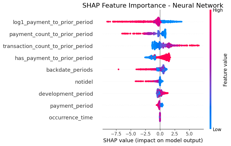
The FFNN relies primarily on recent transaction activity and financial history to drive its predictions. The most influential factor is past payment magnitude (log1_payment_to_prior_period), where higher historical payments systematically pull future expectations down, while lower past values push predictions up. Beyond financial history, the model relies heavily on transaction frequency: higher counts of transactions and payments serve as a strong signal of claim activity, significantly raising predicted values. Secondary variables like reporting delays or claim age play a far more marginal role. The ability of the Neural Network to produce a more smoothed results is reflected in monotonic interpretation of the features, which seems more easy to understand.
Gradient Boosting Machine (GBM) Interpretability
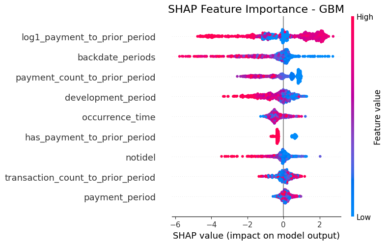
The GBM shifts its reliance heavily toward operational delays and financial magnitude. Unlike the FFNN, its single biggest driver is operational reporting delay (backdate_periods), where extreme delays (red dots) heavily pull down predictions. Past payment magnitude (log1_payment_to_prior_period) remains crucial, but displays a wider, bi-directional spread where high values push predictions significantly in both directions. While transaction counts still contribute to the predictions, their overall impact is far more condensed compared to the neural network, showing that the tree-based model relies more on administrative timelines and financial weight rather than process frequency.
Comparative Insight
Comparing the two SHAP analyses reveals a fundamental difference in how each architecture processes information. The FFNN displays a much clearer and more intuitive feature logic: its top predictors show monotonic trends—such as transaction counts pushing predictions consistently upward, or prior payments pulling them down—resulting in a smooth behavior. This stems directly from the FFNN’s ability to approximate continuous functions through smooth, global optimization.
In contrast, the GBM produces a far more scattered and non-linear pattern, particularly for its main financial driver (log1_payment_to_prior_period), where high values trigger both positive and negative corrections depending on the branch. This highlights how the tree-based architecture relies on sharp, localized split decisions and complex feature interactions, making certain effects more difficult to interpret compared to the smooth representations learned by the Neural Network. This fragmented behavior is the direct outcome of sequential boosting steps and discrete tree partitioning.
Sensitivity Analysis: Alternative Training Strategies
A critical phase of this research involved evaluating how both architectures respond to different data structures. By testing various preprocessing and weighting strategies, we identified the optimal configuration for each model and uncovered fundamental differences in how Neural Networks and GBMs process actuarial history. For simplicity, we focus on the results of the first seed.
To ensure a transparent comparison, we categorized the training environments as follows:
- Static Baseline (
NN_Train): The standard dataset featuring fixed historical snapshots with no dynamic sampling, representing a traditional machine learning approach. Every claim appears only once for each snapshot. - Full Augmented History (
NN_Train_Full): Includes the complete, uncompressed development trajectory for every claim, maximizing the information available for the models to learn the “pathway” of payments. Every claim appears multiple times for each snapshot, but with different backdated information. - Full Augmented History - Optimized Configurations: Full Augmented History but integrating some techniques to handle the claims repeated for each snapshot.
- FFNN - Dynamic Sampling: Our final choice for the Neural Network, which utilizes a dynamic sampling approach to ensure exposure to diverse claim lifecycle stages during training.
- GBM - Weighting Logic: Our final choice for the Gradient Boosting model. This strategy applies a specific weighting logic to the
NN_Train_Fulldataset to ensure structural balance.
AV Error
As previously defined, the AV Error% is a key metric for actuarial evaluation, directly reflecting the accuracy of overall reserve projections.
| Model | Static Baseline | Full Augmented History | Optimized Configuration |
|---|---|---|---|
| FFNN (AV Error %) | 13.06% | 8.65% | 8.31% |
| GBM (AV Error %) | 12.94% | 41.95% | 9.88% |
The results show how data structure directly affects macro-level reserve calibration. When trained on the unweighted Full Augmented History, the GBM suffers a major breakdown, resulting in a 41.95% error with a poor performance despite there are more information available than the standard scenario. The unweighted repetitive snapshots cause tree splits to miscalculate the aggregate portfolio growth, leading to severe systematic bias at ultimate closure. Applying the \(1/n\) weighting strategy resolves this structural issue, bringing the GBM’s ultimate error down to a competitive 9.88%. For the FFNN, performance remains consistently stable across configurations. While both the Full History (8.65%) and Dynamic Sampling (8.31%) yield strong ultimate estimates, the latter was selected as the final strategy because it provides slightly better stability in long-tail projections while reducing computational redundancy. Overall, these findings confirm that the FFNN naturally maintains more macro balance across different data structures, whereas tree-based models require explicit weighting to produce reliable ultimate solvency estimates.
RMSE
The RMSE measures the error on individual incremental payments, serving as an indicator of how precisely the model captures the volatility and “noise” of each specific time step.
| Model | Static Baseline | Full Augmented History | Optimized Configuration |
|---|---|---|---|
| FFNN (RMSE) | 55,000 | 54,894 | 54,913 |
| GBM (RMSE) | 56,809 | 4,022,03 | 57,253 |
The GBM’s performance across these data structures highlights a core architectural limitation, when trained on the unweighted Full Augmented History, the model suffers a complete structural collapse as already observed looking at the AV Error. Applying a simple \(1/n\) weighting logic to each claim snapshot fixes this problem by restoring the original portfolio proportions. Once balanced, the GBM significantly reduces its point-in-time RMSE (57,253), approaching the performance of the FFNN. This demonstrates that boosting can also achieve high precision at a granular level when the training data is properly weighted.
Conclusions
In this study, both machine learning and deep learning models demonstrate a clear predictive advantage over the traditional Chain Ladder. While the Chain Ladder remains a useful benchmark due to its simplicity and low computational overhead, its performance breaks down where there are trends in recent occurrence periods and where data is sparse. In contrast, both the Feed-Forward Neural Network (FFNN) and the Gradient Boosting Machine (GBM) are able to adapt to such emerging trends to a greater extent than the Chain Ladder resulting in better overall performance.
Even if the overall performance of both advanced models remains very similar, the FFNN emerges as the more performant and resilient approach. This is explained by its flexible structure which is able to generate new features which approximate hidden patterns in the data during model training. This allows the neural network to capture the overall evolution of a claim, resulting in smoother predictions and clear, monotonic feature interactions while achieving lower error in both aggregate reserve and ultimate cost estimation.
In contrast the GBM cannot generate new features during training, it can only work with the features provided in the training data from which it constructs discrete decision trees sequentially to correct residual errors. As a result the GBM is sensitive to features provided and the sample density of those features. We observed that, without a dedicated weighting logic, the greedy boosting algorithm will overfit to older occurrence periods which have more training data observations at the expense of more recent occurrence periods.
We observe that the use of backdating in the training data preparation avoids the need for a recursive prediction loop, addressing a common critisism and barrier to the adoption and use of ML techniques in reserving. With the use of SHAP exhibits we can gain useful insights into the key drivers of claim development within the FFNN and GBM models removing another common barrier to adoption.
So should you be adopting the use of FFNN and GBMs in your reserving process?
Well, be aware that there is a class of neural networks that are better structured to learn time series and sequential patterns that are likely to be present in our reserving data. With names like LSTM, GRUs and transformers they are gaining increasing research application to reserving use cases and we intend to cover them in our future blogs. However they are an order more complex than the FFNN and GBM approaches covered here and generally require larger volumes of data and compute power to be effective.
So hopefully you see value in trying the FFNN and GBM approaches, recognizing that the practice you get from doing so will set you up well for a future of using the more complex sequence neural networks that are on the near horizon.