From Chain Ladder to Individual Mixture Density Networks on SPLICE Data

Introduction

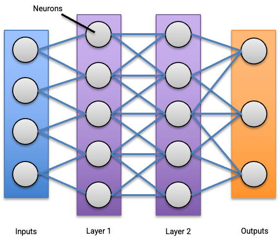
In an upcoming talk I’ll be looking at the use of neural networks in individual claims modelling. I start with a Chain Ladder model and progressively expand it into an deep learning individual claim model while still having sensible results. Additionally, there is a benchmark against a GBM model as well. I use a number of different synthetic data sets for this purpose, the first satisfying Chain Ladder assumptions and the remaining ones breaking these assumptions in different ways.

My talk is supported by 5 freely available Jupyter notebooks for each of the data sets so please refer to these if you want to run the code. These may be downloaded as this zip file

The remainder of this post covers the contents and results of the notebook for data set 5.

The notebook is long but structured into sections as follows:

• Data: Read in SPLICE data (including case estimates) and create additional fields, test and train datasets,
• Chain ladder: Directly calculate Chain Ladder factors as a baseline,
• Chain ladder (GLM) Recreate Chain Ladder results, with a GLM formulation,
• Individual GLM Convert the GLM into a very basic individual claims model,
• Individual GLM with splines Replace the overparametrized one-hot encoding with splines,
• Residual network Consider a ResNet,
• Spline-based individual network: Create a customised neural network architecture with similar behaviour to the individual GLM with splines,
• Spline-based Individual Log-normal Mixture Density Network: Introduce a MDN-based network, with modifications to accommodate a log-normal distribution,
• Rolling origin cross-validation and parameter search,
• Additional data augmentation for training individual claim features,
• Detailed individual models using claim features, including a hyperparameter tuned GBM as a benchmark,
• Review and summary.

dataset_no = 5     # Re-run this for datasets 1-5 to see how it performs
cutoff     = 40    # 40 is the (hard-coded) cut-off as set out previously
cv_runs    = 1     # Testing only: 4, proper runs of the models: 24
glm_iter   = 500   # 500 epochs for gradient descent fitting of GLMs is very quick
nn_iter    = 500   # 100 for experimentation, 500 appears to give models that have fully converged or are close to convergence. 
nn_cv_iter = 100   # Lower for CV to save running time
mdn_iter   = 500   # Latest architecture and loss converges fairly quickly

!pip show pandas numpy scikit-learn torch matplotlib

Name: pandas
Version: 1.5.2
Summary: Powerful data structures for data analysis, time series, and statistics
Home-page: https://pandas.pydata.org
Author: The Pandas Development Team
Author-email: pandas-dev@python.org
License: BSD-3-Clause
Location: /Users/jacky/GitRepos/NNs-on-Individual-Claims/.conda/lib/python3.10/site-packages
Requires: numpy, python-dateutil, pytz
Required-by: catboost, category-encoders, chainladder, cmdstanpy, darts, datasets, nfoursid, pmdarima, prophet, pytorch-tabular, seaborn, shap, statsforecast, statsmodels, xarray
---
Name: numpy
Version: 1.23.5
Summary: NumPy is the fundamental package for array computing with Python.
Home-page: https://www.numpy.org
Author: Travis E. Oliphant et al.
Author-email: 
License: BSD
Location: /Users/jacky/GitRepos/NNs-on-Individual-Claims/.conda/lib/python3.10/site-packages
Requires: 
Required-by: catboost, category-encoders, cmdstanpy, contourpy, darts, datasets, duckdb, lightgbm, matplotlib, nfoursid, numba, pandas, patsy, pmdarima, prophet, pyarrow, pyod, pytorch-lightning, pytorch-tabnet, pytorch-tabular, ray, scikit-learn, scikit-optimize, scipy, seaborn, shap, skorch, sparse, statsforecast, statsmodels, tbats, tensorboard, tensorboardX, torchmetrics, tune-sklearn, xarray, xgboost
---
Name: scikit-learn
Version: 1.2.0
Summary: A set of python modules for machine learning and data mining
Home-page: http://scikit-learn.org
Author: 
Author-email: 
License: new BSD
Location: /Users/jacky/GitRepos/NNs-on-Individual-Claims/.conda/lib/python3.10/site-packages
Requires: joblib, numpy, scipy, threadpoolctl
Required-by: category-encoders, chainladder, darts, lightgbm, pmdarima, pyod, pytorch-tabnet, pytorch-tabular, scikit-optimize, shap, skorch, tbats, tune-sklearn
---
Name: torch
Version: 1.13.1
Summary: Tensors and Dynamic neural networks in Python with strong GPU acceleration
Home-page: https://pytorch.org/
Author: PyTorch Team
Author-email: packages@pytorch.org
License: BSD-3
Location: /Users/jacky/GitRepos/NNs-on-Individual-Claims/.conda/lib/python3.10/site-packages
Requires: typing-extensions
Required-by: darts, pytorch-lightning, pytorch-tabnet, pytorch-tabular, torchmetrics
---
Name: matplotlib
Version: 3.6.2
Summary: Python plotting package
Home-page: https://matplotlib.org
Author: John D. Hunter, Michael Droettboom
Author-email: matplotlib-users@python.org
License: PSF
Location: /Users/jacky/GitRepos/NNs-on-Individual-Claims/.conda/lib/python3.10/site-packages
Requires: contourpy, cycler, fonttools, kiwisolver, numpy, packaging, pillow, pyparsing, python-dateutil
Required-by: catboost, chainladder, darts, nfoursid, prophet, pyod, pytorch-tabular, seaborn, statsforecast

import pandas as pd
import numpy as np
from matplotlib import pyplot as plt

# from torch.utils.data.sampler import BatchSampler, RandomSampler
# from torch.utils.data import DataLoader

import torch
import torch.nn as nn
from torch.nn import functional as F

from torch.autograd import Variable

from sklearn.compose import ColumnTransformer, TransformedTargetRegressor
from sklearn.preprocessing import OneHotEncoder, StandardScaler, MinMaxScaler, SplineTransformer
from sklearn.pipeline import Pipeline

from sklearn.metrics import mean_squared_error

from sklearn.base import BaseEstimator, RegressorMixin, TransformerMixin
from sklearn.utils.validation import check_X_y, check_array, check_is_fitted
from sklearn.ensemble import HistGradientBoostingRegressor

from sklearn.model_selection import GridSearchCV, RandomizedSearchCV, PredefinedSplit
# from skopt import BayesSearchCV
import math

pd.options.display.float_format = '{:,.2f}'.format

Scikit Module

This has been used in past experiments so it is basically my boilerplate code. With minor tweaks.

class TabularNetRegressor(BaseEstimator, RegressorMixin):
    def __init__(
        self, 
        module,
        criterion=nn.PoissonNLLLoss,
        max_iter=100,   
        max_lr=0.01,
        keep_best_model=False,
        batch_function=None,
        rebatch_every_iter=1,
        n_hidden=20,                  
        l1_penalty=0.0,          # lambda is a reserved word
        l1_applies_params=["linear.weight", "hidden.weight"],
        weight_decay=0.0,
        batch_norm=False,
        interactions=True,
        dropout=0.0,
        clip_value=None,
        n_gaussians=3,
        verbose=1,                
        device="cpu" if torch.backends.mps.is_available() else ("cuda" if torch.cuda.is_available() else "cpu"),  # Use GPU if available, leave mps off until more stable
        init_extra=None,
        **kwargs
    ):
        """ Tabular Neural Network Regressor (for Claims Reserving)

        This trains a neural network with specified loss, Log Link and l1 LASSO penalties
        using Pytorch. It has early stopping.

        Args:
            module: pytorch nn.Module. Should have n_input and n_output as parameters and
                if l1_penalty, init_weight, or init_bias are used, a final layer 
                called "linear".

            criterion: pytorch loss function. Consider nn.PoissonNLLLoss for log link.

            max_iter (int): Maximum number of epochs before training stops. 
                Previously this used a high value for triangles since the record count is so small.
                For larger regression problems, a lower number of iterations may be sufficient.

            max_lr (float): Min / Max learning rate - we will use one_cycle_lr

            keep_best_model (bool): If true, keep and use the model weights with the best loss rather 
                than the final weights.

            batch_function (None or fn): If not None, used to get a batch from X and y

            rebatch_every_iter (int): redo batches every

            l1_penalty (float): l1 penalty factor. If not zero, is applied to 
                the layers in the Module with names matching l1_applies_params.

                (we use l1_penalty because lambda is a reserved word in Python 
                for anonymous functions)

            weight_decay (float): weight decay - analogous to l2 penalty factor
                Applied to all weights

            clip_value (None or float): clip gradient norms at a particular value
            
            n_hidden (int), batch_norm(bool), dropout (float), interactions(bool), n_gaussians(int): 
                Passed to module. Hidden layer size, batch normalisation, dropout percentages, and interactions flag.

            init_extra (coerces to torch.Tensor): set init_bias, passed to module. If none, default to np.log(y.mean()).values.astype(np.float32)

            verbose (int): 0 means don't print. 1 means do print.
        """
        self.module = module
        self.criterion = criterion
        self.keep_best_model = keep_best_model
        self.l1_penalty = l1_penalty
        self.l1_applies_params = l1_applies_params
        self.weight_decay = weight_decay
        self.max_iter = max_iter
        self.n_hidden = n_hidden
        self.batch_norm = batch_norm
        self.batch_function = batch_function
        self.rebatch_every_iter = rebatch_every_iter
        self.interactions = interactions
        self.dropout = dropout
        self.n_gaussians = n_gaussians
        self.device = device
        self.target_device = torch.device(device)    
        self.max_lr = max_lr
        self.init_extra = init_extra
        self.print_loss_every_iter = max(1, int(max_iter / 10))
        self.verbose = verbose
        self.clip_value = clip_value
        self.kwargs = kwargs

        
    def fix_array(self, y):
        "Need to be picky about array formats"
        if isinstance(y, pd.DataFrame) or isinstance(y, pd.Series):
            y = y.values
        if y.ndim == 1:
            y = y.reshape(-1, 1)
        y = y.astype(np.float32)
        return y
        

    def setup_module(self, n_input, n_output):
         
        # Training new model
        self.module_ = self.module(
            n_input=n_input, 
            n_output=n_output,
            n_hidden=self.n_hidden,
            batch_norm=self.batch_norm,
            dropout=self.dropout,
            interactions_trainable=self.interactions,
            n_gaussians=self.n_gaussians,
            init_bias=self.init_bias_calc,
            init_extra=self.init_extra,
            **self.kwargs
        ).to(self.target_device)
        

    def fit(self, X, y):
        # The main fit logic is in partial_fit
        # We will try a few times if numbers explode because NN's are finicky and we are doing CV
        n_input = X.shape[-1]
        n_output = 1 if y.ndim == 1 else y.shape[-1]
        self.init_bias_calc = np.log(y.mean()).values.astype(np.float32)
        self.setup_module(n_input=n_input, n_output=n_output)

        # Partial fit means you take an existing model and keep training 
        # so the logic is basically the same
        self.partial_fit(X, y)

        return self


    def partial_fit(self, X, y):
        # Check that X and y have correct shape
        X, y = check_X_y(X, y, multi_output=True)

        # Convert to Pytorch Tensor
        X_tensor = torch.from_numpy(self.fix_array(X)).to(self.target_device)
        y_tensor = torch.from_numpy(self.fix_array(y)).to(self.target_device)

        # Optimizer - the generically useful AdamW. Other options like SGD
        # are also possible.
        optimizer = torch.optim.AdamW(
            params=self.module_.parameters(),
            lr=self.max_lr / 10,
            weight_decay=self.weight_decay
        )
        
        # Scheduler - one cycle LR
        scheduler = torch.optim.lr_scheduler.OneCycleLR(
            optimizer, 
            max_lr=self.max_lr, 
            steps_per_epoch=1, 
            epochs=self.max_iter
        )

        # Loss Function
        try:
            loss_fn = self.criterion(log_input=False).to(self.target_device)  # Pytorch loss function
        except TypeError:
            loss_fn = self.criterion  # Custom loss function

        best_loss = float('inf') # set to infinity initially

        if self.batch_function is not None:
            X_tensor_batch, y_tensor_batch = self.batch_function(X_tensor, y_tensor)
        else:
            X_tensor_batch, y_tensor_batch = X_tensor, y_tensor

        # Training loop
        for epoch in range(self.max_iter):   # Repeat max_iter times

            self.module_.train()
            y_pred = self.module_(X_tensor_batch)  #  Apply current model

            loss = loss_fn(y_pred, y_tensor_batch) #  What is the loss on it?
            if self.l1_penalty > 0.0:        #  Lasso penalty
                loss += self.l1_penalty * sum(
                    [
                        w.abs().sum()
                        for p, w in self.module_.named_parameters()
                        if p in self.l1_applies_params
                    ]
                )

            if self.keep_best_model & (loss.item() < best_loss):
                best_loss = loss.item()
                self.best_model = self.module_.state_dict()

            optimizer.zero_grad()            #  Reset optimizer
            loss.backward()                  #  Apply back propagation

            # gradient norm clipping
            if self.clip_value is not None:
                grad_norm = torch.nn.utils.clip_grad_norm_(self.module_.parameters(), self.clip_value)
                # check if gradients have been clipped
                if (self.verbose >= 2) & (grad_norm > self.clip_value):
                    print(f'Gradient norms have been clipped in epoch {epoch}, value before clipping: {grad_norm}')    

            optimizer.step()                 #  Update model parameters
            scheduler.step()

            if torch.isnan(loss.data).tolist():
                raise ValueError('Error: nan loss')


            # Every self.print_loss_every_iter steps, print RMSE 
            if (epoch % self.print_loss_every_iter == 0) and (self.verbose > 0):
                self.module_.eval()                     # Eval mode 
                self.module_.point_estimates=True       # Distributional models - set to point                
                y_pred_point = self.module_(X_tensor)   # Get "real" model estimates
                assert(y_pred_point.size() == y_tensor.size())
                rmse = torch.sqrt(torch.mean(torch.square(y_pred_point - y_tensor)))
                self.module_.train()                     # back to training
                self.module_.point_estimates=False       # Distributional models - set to point
                
                print("Train RMSE: ", rmse.data.tolist(), " Train Loss: ", loss.data.tolist())

            if (self.batch_function is not None) & (epoch % self.rebatch_every_iter == 0):
                print(f"refreshing batch on epoch {epoch}")
                X_tensor_batch, y_tensor_batch = self.batch_function(X_tensor, y_tensor)
        
        if self.keep_best_model:
            self.module_.load_state_dict(self.best_model)
            self.module_.eval()

        # Return the regressor
        return self


    def predict(self, X, point_estimates=True):
        # Checks
        check_is_fitted(self)      # Check is fit had been called
        X = check_array(X)         # Check input

        # Convert to Pytorch Tensor
        X_tensor = torch.from_numpy(self.fix_array(X)).to(self.target_device)
      
        self.module_.eval()  # Eval (prediction) mode
        self.module_.point_estimates = point_estimates

        # Apply current model and convert back to numpy
        if point_estimates:
            y_pred = self.module_(X_tensor).cpu().detach().numpy()
            if y_pred.shape[-1] == 1: 
                return y_pred.ravel()
            else:
                return y_pred
        else:
            y_pred = self.module_(X_tensor)
            return y_pred


    def score(self, X, y):
        # Negative RMSE score (higher needs to be better)
        y_pred = self.predict(X)
        y = self.fix_array(y)
        return -np.sqrt(np.mean((y_pred - y)**2))

class ColumnKeeper(BaseEstimator, TransformerMixin):
    """Keeps named cols, preserves DataFrame output"""
    def __init__(self, cols):
        self.cols = cols

    def fit(self, X, y):
        return self

    def transform(self, X):
        return X.copy()[self.cols]

Data

Convert to a time series with one record per time period (even if multiple or no claims transactions). This follows my earlier gist here but rewritten in pure pandas (shorter, less dependencies, but probably less readable so refer to gist for the concepts).

paid = pd.read_csv(f"https://raw.githubusercontent.com/agi-lab/SPLICE/main/datasets/complexity_{dataset_no}/payment_{dataset_no}.csv")
incurred = pd.read_csv(f"https://raw.githubusercontent.com/agi-lab/SPLICE/main/datasets/complexity_{dataset_no}/incurred_{dataset_no}.csv")

# Recreate some of the columns from paid into the incurred set
incurred.loc[:, "trn_no"] = incurred.groupby("claim_no").cumcount() + 1
incurred.loc[incurred.txn_type.str.contains("P"), "pmt_no"] = incurred.loc[incurred.txn_type.str.contains("P")].groupby("claim_no").cumcount() + 1
incurred["payment_period"] = np.ceil(incurred.txn_time).astype("int")
incurred["payment_size"] = incurred.groupby("claim_no").cumpaid.diff()
incurred["payment_size"] = incurred["payment_size"].fillna(incurred["cumpaid"])
incurred["incurred_incremental"] = incurred.groupby("claim_no").incurred.diff()
incurred["incurred_incremental"] = incurred["incurred_incremental"].fillna(incurred["incurred"])
transactions = incurred.merge(
    paid[["claim_no", "occurrence_period", "occurrence_time", "notidel", "setldel"]].drop_duplicates(),
    on="claim_no",
)
transactions["noti_period"] = np.ceil(transactions["occurrence_time"] + transactions["notidel"]).astype('int')
transactions["settle_period"] = np.ceil(transactions["occurrence_time"] + transactions["notidel"] + transactions["setldel"]).astype('int')

# Apply cut-off since some of the logic in this notebook assumes an equal set of dimensions
transactions["development_period"] = np.minimum(transactions["payment_period"] - transactions["occurrence_period"], cutoff)  
num_dev_periods = cutoff - 1  # (transactions["payment_period"] - transactions["occurrence_period"]).max()
transactions.head()

	Unnamed: 0	claim_no	claim_size	txn_time	txn_delay	txn_type	incurred	OCL	cumpaid	multiplier	...	payment_period	payment_size	incurred_incremental	occurrence_period	occurrence_time	notidel	setldel	noti_period	settle_period	development_period
0	1	1	232,310.09	1.87	0.00	Ma	31,291.71	31,291.71	0.00	1.00	...	2	0.00	31,291.71	1	0.73	1.13	32.37	2	35	1
1	2	1	232,310.09	7.35	5.49	P	31,291.71	17,575.20	13,716.51	NaN	...	8	13,716.51	0.00	1	0.73	1.13	32.37	2	35	7
2	3	1	232,310.09	13.99	12.12	PMi	32,133.97	1,606.70	30,527.27	0.94	...	14	16,810.76	842.26	1	0.73	1.13	32.37	2	35	13
3	4	1	232,310.09	14.23	12.36	Ma	133,072.86	102,545.59	30,527.27	7.75	...	15	0.00	100,938.89	1	0.73	1.13	32.37	2	35	14
4	5	1	232,310.09	14.41	12.54	Ma	314,565.32	284,038.05	30,527.27	2.36	...	15	0.00	181,492.46	1	0.73	1.13	32.37	2	35	14

5 rows × 22 columns

# Transactions summarised by claim/dev:
transactions_group = (transactions
        .groupby(["claim_no", "development_period"], as_index=False)
        .agg({"payment_size": "sum", "incurred_incremental": "sum", "pmt_no": "max", "trn_no": "max"})
        .sort_values(by=["claim_no", "development_period"])
)

# This is varied from the original version:
range_payment_delay = pd.DataFrame.from_dict({"development_period": range(0, num_dev_periods + 1)})

# Claims header + development periods
claim_head_expand_dev = (
    transactions
    .loc[:, ["claim_no", "occurrence_period", "occurrence_time", "noti_period", "notidel", "settle_period"]]
    .drop_duplicates()
).merge(
    range_payment_delay,
    how="cross"
).assign(
    payment_period=lambda df: (df.occurrence_period + df.development_period),
    is_settled=lambda df: (df.occurrence_period + df.development_period) >= df.settle_period
)

# create the dataset
dat = claim_head_expand_dev.merge(
    transactions_group,
    how="left",
    on=["claim_no", "development_period"],
).fillna(0)

# Only periods after notification
dat = dat.loc[dat.payment_period >= dat.noti_period]

# Clean close to zero values
dat["payment_size"] = np.where(abs(dat.payment_size) < 1e-2, 0.0, dat.payment_size)

# Cumulative payments
dat["payment_size_cumulative"] = dat[["claim_no", "payment_size"]].groupby('claim_no').cumsum()
dat["incurred_cumulative"] = dat[["claim_no", "incurred_incremental"]].groupby('claim_no').cumsum()
dat["outstanding_claims"] = dat["incurred_cumulative"] - dat["payment_size_cumulative"]
dat["outstanding_claims"] = np.where(abs(dat.outstanding_claims) < 1e-2, 0.0, dat.outstanding_claims)

dat["payment_to_prior_period"] = dat["payment_size_cumulative"] - dat["payment_size"]
dat["has_payment_to_prior_period"] = np.where(dat.payment_to_prior_period > 1e-2, 1, 0)
dat["log1_payment_to_prior_period"] = np.log1p(dat.payment_to_prior_period)

dat["incurred_to_prior_period"] = dat["incurred_cumulative"] - dat["incurred_incremental"]
dat["has_incurred_to_prior_period"] = np.where(dat.incurred_to_prior_period > 1e-2, 1, 0)
dat["log1_incurred_to_prior_period"] = np.log1p(dat.incurred_to_prior_period)

dat["outstanding_to_prior_period"] = dat["incurred_to_prior_period"] - dat["payment_to_prior_period"]
dat["outstanding_to_prior_period"] = np.where(abs(dat.outstanding_to_prior_period) < 1e-2, 0.0, dat.outstanding_to_prior_period)

dat["log1_outstanding_to_prior_period"] = np.log1p(dat.outstanding_to_prior_period)
dat["has_outstanding_to_prior_period"] = np.where(dat.outstanding_to_prior_period > 1e-2, 1, 0)

dat["pmt_no"] = dat.groupby("claim_no")["pmt_no"].cummax()
dat["trn_no"] = dat.groupby("claim_no")["trn_no"].cummax()
dat["payment_count_to_prior_period"] = dat.groupby("claim_no")["pmt_no"].shift(1).fillna(0)
dat["transaction_count_to_prior_period"] = dat.groupby("claim_no")["trn_no"].shift(1).fillna(0)

dat["data_as_at_development_period"] = dat.development_period  # See data augmentation section
dat["backdate_periods"] = 0
dat["payment_period_as_at"] = dat.payment_period

# Potential features for model later:
data_cols = [
    "notidel", 
    "occurrence_time", 
    "development_period", 
    "payment_period", 
    "has_payment_to_prior_period",
    "log1_payment_to_prior_period",
    "has_incurred_to_prior_period",
    "log1_incurred_to_prior_period",
    "has_outstanding_to_prior_period",
    "log1_outstanding_to_prior_period",
    "payment_count_to_prior_period",
    "transaction_count_to_prior_period"]

# The notebook is created on an MacBook Pro M1, which supports GPU mode in float32 only.
dat[dat.select_dtypes(np.float64).columns] = dat.select_dtypes(np.float64).astype(np.float32)

dat["train_ind"] = (dat.payment_period <= cutoff)
dat["cv_ind"] = dat.payment_period % 5  # Cross validate on this column
dat

	claim_no	occurrence_period	occurrence_time	noti_period	notidel	settle_period	development_period	payment_period	is_settled	payment_size	...	outstanding_to_prior_period	log1_outstanding_to_prior_period	has_outstanding_to_prior_period	payment_count_to_prior_period	transaction_count_to_prior_period	data_as_at_development_period	backdate_periods	payment_period_as_at	train_ind	cv_ind
1	1	1	0.73	2	1.13	35	1	2	False	0.00	...	0.00	0.00	0	0.00	0.00	1	0	2	True	2
2	1	1	0.73	2	1.13	35	2	3	False	0.00	...	31,291.71	10.35	1	0.00	1.00	2	0	3	True	3
3	1	1	0.73	2	1.13	35	3	4	False	0.00	...	31,291.71	10.35	1	0.00	1.00	3	0	4	True	4
4	1	1	0.73	2	1.13	35	4	5	False	0.00	...	31,291.71	10.35	1	0.00	1.00	4	0	5	True	0
5	1	1	0.73	2	1.13	35	5	6	False	0.00	...	31,291.71	10.35	1	0.00	1.00	5	0	6	True	1
...	...	...	...	...	...	...	...	...	...	...	...	...	...	...	...	...	...	...	...	...	...
146515	3663	40	39.87	46	5.27	56	35	75	True	0.00	...	0.00	0.00	0	6.00	9.00	35	0	75	False	0
146516	3663	40	39.87	46	5.27	56	36	76	True	0.00	...	0.00	0.00	0	6.00	9.00	36	0	76	False	1
146517	3663	40	39.87	46	5.27	56	37	77	True	0.00	...	0.00	0.00	0	6.00	9.00	37	0	77	False	2
146518	3663	40	39.87	46	5.27	56	38	78	True	0.00	...	0.00	0.00	0	6.00	9.00	38	0	78	False	3
146519	3663	40	39.87	46	5.27	56	39	79	True	0.00	...	0.00	0.00	0	6.00	9.00	39	0	79	False	4

138644 rows × 32 columns

dat.head(10)

	claim_no	occurrence_period	occurrence_time	noti_period	notidel	settle_period	development_period	payment_period	is_settled	payment_size	...	outstanding_to_prior_period	log1_outstanding_to_prior_period	has_outstanding_to_prior_period	payment_count_to_prior_period	transaction_count_to_prior_period	data_as_at_development_period	backdate_periods	payment_period_as_at	train_ind	cv_ind
1	1	1	0.73	2	1.13	35	1	2	False	0.00	...	0.00	0.00	0	0.00	0.00	1	0	2	True	2
2	1	1	0.73	2	1.13	35	2	3	False	0.00	...	31,291.71	10.35	1	0.00	1.00	2	0	3	True	3
3	1	1	0.73	2	1.13	35	3	4	False	0.00	...	31,291.71	10.35	1	0.00	1.00	3	0	4	True	4
4	1	1	0.73	2	1.13	35	4	5	False	0.00	...	31,291.71	10.35	1	0.00	1.00	4	0	5	True	0
5	1	1	0.73	2	1.13	35	5	6	False	0.00	...	31,291.71	10.35	1	0.00	1.00	5	0	6	True	1
6	1	1	0.73	2	1.13	35	6	7	False	0.00	...	31,291.71	10.35	1	0.00	1.00	6	0	7	True	2
7	1	1	0.73	2	1.13	35	7	8	False	13,716.51	...	31,291.71	10.35	1	0.00	1.00	7	0	8	True	3
8	1	1	0.73	2	1.13	35	8	9	False	0.00	...	17,575.20	9.77	1	1.00	2.00	8	0	9	True	4
9	1	1	0.73	2	1.13	35	9	10	False	0.00	...	17,575.20	9.77	1	1.00	2.00	9	0	10	True	0
10	1	1	0.73	2	1.13	35	10	11	False	0.00	...	17,575.20	9.77	1	1.00	2.00	10	0	11	True	1

10 rows × 32 columns

Train test split is set up by payment period - past vs future.

There is a caveat for an unrealistic assumption - there is one record per claim even if it is reported “in the future” past the cutoff.

This affects the model training and it does mean when looking at aggregate prediction data that the model knows what the ultimate count is.

However, normally when we are building individual claim models they are used to predict expected costs of known claims so this is not a huge issue.

Chain Ladder, Direct Calculation, Aggregated Data

Chain ladder calculation, from first principles. Based on this article

triangle = (dat
    .groupby(["occurrence_period", "development_period", "payment_period"], as_index=False)
    .agg({"payment_size_cumulative": "sum", "payment_size": "sum"})
    .sort_values(by=["occurrence_period", "development_period"])
)
triangle_train = triangle.loc[triangle.payment_period <= cutoff]
triangle_test = triangle.loc[triangle.payment_period > cutoff]

triangle_train.pivot(index = "occurrence_period", columns = "development_period", values = "payment_size_cumulative")

development_period	0	1	2	3	4	5	6	7	8	9	...	30	31	32	33	34	35	36	37	38	39
occurrence_period
1	0.00	31,551.25	152,793.12	680,415.06	1,650,518.75	1,932,605.62	2,602,592.25	3,222,089.50	3,775,028.25	4,788,738.50	...	15,739,832.00	16,082,119.00	16,780,246.00	17,400,658.00	17,422,826.00	17,422,826.00	17,485,892.00	17,485,892.00	17,485,892.00	17,485,892.00
2	10,286.75	49,493.38	132,020.67	430,670.75	1,225,081.75	2,044,801.12	2,433,025.00	2,808,325.75	3,586,153.00	4,218,801.50	...	14,386,516.00	14,880,894.00	15,342,595.00	15,378,178.00	15,378,178.00	15,409,743.00	15,409,743.00	15,433,019.00	15,795,103.00	NaN
3	0.00	62,389.38	640,980.81	987,640.00	1,536,782.25	2,385,404.00	3,177,442.25	3,698,036.50	3,918,063.50	4,333,062.00	...	15,336,449.00	15,437,039.00	15,646,281.00	15,867,258.00	16,067,564.00	16,067,564.00	16,071,147.00	16,108,434.00	NaN	NaN
4	5,646.32	63,203.44	245,984.03	584,083.62	1,030,191.31	2,371,411.75	3,179,435.75	4,964,554.00	6,244,163.00	6,612,675.00	...	17,058,208.00	17,107,564.00	17,202,888.00	17,256,650.00	17,256,650.00	17,598,124.00	18,155,534.00	NaN	NaN	NaN
5	0.00	22,911.55	177,779.52	431,647.50	872,805.94	1,619,887.00	2,862,273.00	3,462,464.75	4,956,769.50	6,237,362.50	...	19,066,434.00	19,121,178.00	19,157,450.00	19,222,538.00	19,222,538.00	19,235,524.00	NaN	NaN	NaN	NaN
6	2,259.24	62,889.91	357,107.84	813,191.12	1,218,815.75	2,030,866.88	3,065,646.00	4,652,615.50	5,097,719.50	6,097,211.00	...	21,011,932.00	21,511,248.00	21,511,248.00	21,511,248.00	21,611,440.00	NaN	NaN	NaN	NaN	NaN
7	25,200.05	212,996.06	303,872.44	522,915.66	1,180,820.88	3,314,907.25	3,931,794.25	4,110,920.00	5,112,089.00	5,522,927.00	...	17,723,798.00	18,120,490.00	18,120,490.00	18,526,526.00	NaN	NaN	NaN	NaN	NaN	NaN
8	0.00	101,324.27	482,201.94	1,302,672.88	1,762,479.38	2,816,009.75	3,599,199.00	4,404,539.50	5,549,806.50	6,296,549.50	...	27,771,816.00	27,771,816.00	27,839,500.00	NaN	NaN	NaN	NaN	NaN	NaN	NaN
9	0.00	21,563.11	207,902.11	1,019,339.94	1,467,485.12	2,183,192.50	2,792,763.75	3,155,922.75	4,188,714.25	5,294,733.50	...	19,726,484.00	19,798,286.00	NaN	NaN	NaN	NaN	NaN	NaN	NaN	NaN
10	0.00	62,438.00	642,477.19	1,220,443.88	1,512,127.75	2,125,860.75	3,205,997.25	5,542,220.00	6,233,909.50	7,278,581.00	...	23,628,224.00	NaN	NaN	NaN	NaN	NaN	NaN	NaN	NaN	NaN
11	6,573.56	233,421.70	858,658.38	1,487,226.75	2,326,138.75	4,001,959.50	4,689,719.00	5,703,576.50	7,421,133.00	8,338,611.50	...	NaN	NaN	NaN	NaN	NaN	NaN	NaN	NaN	NaN	NaN
12	0.00	337,785.12	602,649.94	947,861.81	1,960,324.38	2,438,331.25	3,263,283.25	4,443,729.00	4,600,126.00	4,950,643.00	...	NaN	NaN	NaN	NaN	NaN	NaN	NaN	NaN	NaN	NaN
13	0.00	48,432.94	257,028.44	713,263.12	1,489,202.25	2,399,702.50	3,479,596.75	4,570,094.00	5,228,066.00	8,120,785.50	...	NaN	NaN	NaN	NaN	NaN	NaN	NaN	NaN	NaN	NaN
14	18,463.75	352,189.09	1,015,863.62	1,451,495.75	2,553,104.25	3,266,427.50	5,020,334.00	6,462,674.00	8,515,544.00	9,761,134.00	...	NaN	NaN	NaN	NaN	NaN	NaN	NaN	NaN	NaN	NaN
15	0.00	64,434.53	272,821.25	689,155.88	1,832,749.12	3,660,129.75	4,680,136.50	7,358,847.00	9,028,388.00	10,283,629.00	...	NaN	NaN	NaN	NaN	NaN	NaN	NaN	NaN	NaN	NaN
16	172,118.23	276,003.81	1,468,529.00	2,473,900.50	3,320,296.25	4,172,269.25	6,421,418.50	7,663,898.50	9,201,556.00	9,852,889.00	...	NaN	NaN	NaN	NaN	NaN	NaN	NaN	NaN	NaN	NaN
17	0.00	115,323.28	533,563.88	1,628,512.75	3,782,490.00	5,496,876.00	7,221,503.00	8,019,986.00	8,644,119.00	9,252,501.00	...	NaN	NaN	NaN	NaN	NaN	NaN	NaN	NaN	NaN	NaN
18	0.00	113,693.24	534,180.81	1,126,199.38	2,086,124.12	2,636,258.50	3,415,784.25	4,550,892.50	6,384,181.50	7,276,585.00	...	NaN	NaN	NaN	NaN	NaN	NaN	NaN	NaN	NaN	NaN
19	0.00	65,176.80	593,353.38	1,377,092.75	2,679,311.25	4,561,606.50	5,190,826.50	6,896,302.50	7,889,414.50	10,040,150.00	...	NaN	NaN	NaN	NaN	NaN	NaN	NaN	NaN	NaN	NaN
20	3,269.31	303,522.59	789,422.50	1,556,370.50	2,431,901.50	4,251,400.00	6,718,960.50	9,005,605.00	10,659,464.00	12,031,561.00	...	NaN	NaN	NaN	NaN	NaN	NaN	NaN	NaN	NaN	NaN
21	0.00	99,668.09	1,164,366.00	1,829,524.38	3,262,251.50	4,136,417.75	5,829,693.00	7,624,765.00	9,753,255.00	11,093,190.00	...	NaN	NaN	NaN	NaN	NaN	NaN	NaN	NaN	NaN	NaN
22	0.00	73,295.09	370,612.00	1,025,605.56	2,284,124.00	3,889,548.75	5,347,188.00	6,029,389.00	7,281,124.50	8,422,002.00	...	NaN	NaN	NaN	NaN	NaN	NaN	NaN	NaN	NaN	NaN
23	738,959.81	944,850.44	1,558,499.88	2,354,515.50	4,080,220.25	6,339,416.00	7,833,012.00	9,289,169.00	11,375,192.00	12,184,491.00	...	NaN	NaN	NaN	NaN	NaN	NaN	NaN	NaN	NaN	NaN
24	32,878.80	139,590.50	722,637.12	2,000,021.75	3,699,119.00	4,275,938.50	5,317,856.00	7,233,627.50	8,291,626.50	8,943,028.00	...	NaN	NaN	NaN	NaN	NaN	NaN	NaN	NaN	NaN	NaN
25	0.00	67,300.14	794,740.44	1,203,488.25	1,704,533.00	2,902,497.25	3,623,180.75	4,985,555.50	6,397,038.50	7,434,320.50	...	NaN	NaN	NaN	NaN	NaN	NaN	NaN	NaN	NaN	NaN
26	0.00	222,579.27	724,894.44	1,461,998.50	2,063,614.62	3,727,648.00	6,192,158.00	7,523,790.50	8,246,265.50	10,140,250.00	...	NaN	NaN	NaN	NaN	NaN	NaN	NaN	NaN	NaN	NaN
27	0.00	21,265.95	431,409.00	1,352,109.50	2,414,385.00	3,756,162.50	4,874,574.00	8,397,044.00	10,588,447.00	11,796,448.00	...	NaN	NaN	NaN	NaN	NaN	NaN	NaN	NaN	NaN	NaN
28	0.00	281,462.16	1,313,574.88	2,223,132.25	3,606,104.75	5,205,782.00	8,583,559.00	9,386,136.00	12,726,494.00	14,633,823.00	...	NaN	NaN	NaN	NaN	NaN	NaN	NaN	NaN	NaN	NaN
29	109,492.41	749,180.50	2,196,492.25	3,589,296.25	5,510,728.00	7,582,901.50	9,060,910.00	12,036,241.00	14,089,931.00	16,412,483.00	...	NaN	NaN	NaN	NaN	NaN	NaN	NaN	NaN	NaN	NaN
30	0.00	152,130.56	1,171,098.38	2,392,989.25	4,038,955.50	5,796,675.50	6,487,593.00	7,935,940.00	9,448,145.00	12,658,112.00	...	NaN	NaN	NaN	NaN	NaN	NaN	NaN	NaN	NaN	NaN
31	0.00	102,149.25	587,694.50	1,739,223.50	3,054,168.25	4,391,554.00	6,488,115.50	8,532,481.00	9,589,075.00	13,596,397.00	...	NaN	NaN	NaN	NaN	NaN	NaN	NaN	NaN	NaN	NaN
32	0.00	137,841.00	841,636.31	1,810,914.25	3,203,533.50	4,339,657.00	7,193,541.50	8,792,350.00	11,048,168.00	NaN	...	NaN	NaN	NaN	NaN	NaN	NaN	NaN	NaN	NaN	NaN
33	0.00	134,954.59	1,254,893.38	2,674,034.25	4,403,876.00	5,591,899.50	6,810,711.50	8,387,086.00	NaN	NaN	...	NaN	NaN	NaN	NaN	NaN	NaN	NaN	NaN	NaN	NaN
34	38,893.38	652,741.81	1,456,564.38	2,050,356.00	3,044,004.00	4,796,483.00	7,570,764.00	NaN	NaN	NaN	...	NaN	NaN	NaN	NaN	NaN	NaN	NaN	NaN	NaN	NaN
35	0.00	167,482.09	926,322.88	2,872,798.50	5,040,902.00	6,421,425.50	NaN	NaN	NaN	NaN	...	NaN	NaN	NaN	NaN	NaN	NaN	NaN	NaN	NaN	NaN
36	21,154.29	320,832.66	1,568,433.12	2,393,324.00	4,121,508.50	NaN	NaN	NaN	NaN	NaN	...	NaN	NaN	NaN	NaN	NaN	NaN	NaN	NaN	NaN	NaN
37	83,818.48	819,248.56	1,881,916.25	3,489,761.75	NaN	NaN	NaN	NaN	NaN	NaN	...	NaN	NaN	NaN	NaN	NaN	NaN	NaN	NaN	NaN	NaN
38	28,038.49	216,292.89	1,041,738.56	NaN	NaN	NaN	NaN	NaN	NaN	NaN	...	NaN	NaN	NaN	NaN	NaN	NaN	NaN	NaN	NaN	NaN
39	0.00	237,799.91	NaN	NaN	NaN	NaN	NaN	NaN	NaN	NaN	...	NaN	NaN	NaN	NaN	NaN	NaN	NaN	NaN	NaN	NaN
40	0.00	NaN	NaN	NaN	NaN	NaN	NaN	NaN	NaN	NaN	...	NaN	NaN	NaN	NaN	NaN	NaN	NaN	NaN	NaN	NaN

40 rows × 40 columns

(triangle_train
    .pivot(index = "development_period", columns = "occurrence_period", values = "payment_size_cumulative")
    .plot(logy=True)
)
plt.legend(loc="lower center", bbox_to_anchor=(0.5, -0.8), ncol=5)
plt.title("Training Set, Cumulative Claims by Development Period, Log Scale")

Text(0.5, 1.0, 'Training Set, Cumulative Claims by Development Period, Log Scale')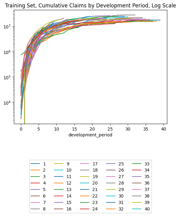

### Get the diagonals in the cumulative IBNR triangle, which represents cumulative payments for a particular
### occurrence period
triangle_diagonal_interim = triangle['payment_size_cumulative'][triangle['payment_period'] == cutoff].reset_index(drop = True)
triangle_diagonal_interim = pd.DataFrame(triangle_diagonal_interim).rename(columns = {'payment_size_cumulative': 'diagonal'})
triangle_diagonal = triangle_diagonal_interim.iloc[::-1].reset_index(drop = True)

### Sum cumulative payments by development period - to be used to calculate CDFs later
development_period_sum_interim = triangle_train.groupby(by = 'development_period').sum()
development_period_sum = development_period_sum_interim['payment_size_cumulative'].reset_index(drop = True)
development_period_sum = pd.DataFrame(development_period_sum).rename(columns = {'payment_size_cumulative': 'dev_period_sum'})

# Merge two dataframes
df_cdf = pd.concat([triangle_diagonal, development_period_sum], axis = 1)

## dev_period_sum_alt column is to ensure the claims for two consecutive periods have the same number
## of levels/elements (and division of these two claims columns give the CDF)
df_cdf['dev_period_sum_alt'] = df_cdf['dev_period_sum'] - df_cdf['diagonal']

### Calculate Development Factors
df_cdf['dev_period_sum_shift'] = df_cdf['dev_period_sum'].shift(-1)
df_cdf['development_factor'] = df_cdf['dev_period_sum_shift'] / df_cdf['dev_period_sum_alt']
df_cdf['factor_to_ultimate'] = df_cdf.sort_index(ascending=False).fillna(1.0).development_factor.cumprod()
df_cdf['percentage_of_ultimate'] = 1 / df_cdf['factor_to_ultimate']
df_cdf['incr_perc_of_ultimate'] = df_cdf['percentage_of_ultimate'].diff()
df_cdf

	diagonal	dev_period_sum	dev_period_sum_alt	dev_period_sum_shift	development_factor	factor_to_ultimate	percentage_of_ultimate	incr_perc_of_ultimate
0	0.00	1,297,052.88	1,297,052.88	8,141,409.00	6.28	923.86	0.00	NaN
1	237,799.91	8,141,409.00	7,903,609.00	30,276,714.00	3.83	147.19	0.01	0.01
2	1,041,738.56	30,276,714.00	29,234,976.00	57,907,192.00	1.98	38.42	0.03	0.02
3	3,489,761.75	57,907,192.00	54,417,432.00	93,450,776.00	1.72	19.40	0.05	0.03
4	4,121,508.50	93,450,776.00	89,329,264.00	132,863,912.00	1.49	11.30	0.09	0.04
5	6,421,425.50	132,863,912.00	126,442,488.00	172,164,592.00	1.36	7.59	0.13	0.04
6	7,570,764.00	172,164,592.00	164,593,824.00	210,850,864.00	1.28	5.58	0.18	0.05
7	8,387,086.00	210,850,864.00	202,463,776.00	245,069,168.00	1.21	4.35	0.23	0.05
8	11,048,168.00	245,069,168.00	234,020,992.00	273,903,680.00	1.17	3.60	0.28	0.05
9	13,596,397.00	273,903,680.00	260,307,280.00	298,338,624.00	1.15	3.07	0.33	0.05
10	13,984,095.00	298,338,624.00	284,354,528.00	311,596,960.00	1.10	2.68	0.37	0.05
11	18,247,140.00	311,596,960.00	293,349,824.00	324,199,360.00	1.11	2.45	0.41	0.04
12	20,606,538.00	324,199,360.00	303,592,832.00	331,724,640.00	1.09	2.21	0.45	0.04
13	19,192,766.00	331,724,640.00	312,531,872.00	335,702,112.00	1.07	2.03	0.49	0.04
14	14,057,512.00	335,702,112.00	321,644,608.00	340,176,128.00	1.06	1.89	0.53	0.04
15	13,656,915.00	340,176,128.00	326,519,200.00	348,353,504.00	1.07	1.78	0.56	0.03
16	18,047,780.00	348,353,504.00	330,305,728.00	348,470,784.00	1.05	1.67	0.60	0.04
17	20,920,498.00	348,470,784.00	327,550,272.00	350,782,240.00	1.07	1.58	0.63	0.03
18	18,409,002.00	350,782,240.00	332,373,248.00	350,120,704.00	1.05	1.48	0.68	0.04
19	23,882,838.00	350,120,704.00	326,237,856.00	338,951,584.00	1.04	1.40	0.71	0.04
20	23,967,498.00	338,951,584.00	314,984,096.00	322,580,384.00	1.02	1.35	0.74	0.03
21	20,525,112.00	322,580,384.00	302,055,264.00	309,189,504.00	1.02	1.32	0.76	0.02
22	18,259,918.00	309,189,504.00	290,929,600.00	298,672,864.00	1.03	1.29	0.78	0.02
23	20,473,130.00	298,672,864.00	278,199,744.00	285,398,368.00	1.03	1.26	0.80	0.02
24	19,147,944.00	285,398,368.00	266,250,432.00	273,799,296.00	1.03	1.22	0.82	0.02
25	25,963,162.00	273,799,296.00	247,836,128.00	253,648,528.00	1.02	1.19	0.84	0.02
26	17,040,986.00	253,648,528.00	236,607,536.00	243,831,648.00	1.03	1.16	0.86	0.02
27	24,036,898.00	243,831,648.00	219,794,752.00	222,414,336.00	1.01	1.13	0.89	0.03
28	15,848,811.00	222,414,336.00	206,565,520.00	212,487,168.00	1.03	1.12	0.90	0.01
29	24,596,934.00	212,487,168.00	187,890,240.00	191,449,696.00	1.02	1.08	0.92	0.03
30	23,628,224.00	191,449,696.00	167,821,472.00	169,830,640.00	1.01	1.06	0.94	0.02
31	19,798,286.00	169,830,640.00	150,032,352.00	151,600,704.00	1.01	1.05	0.95	0.01
32	27,839,500.00	151,600,704.00	123,761,200.00	125,163,056.00	1.01	1.04	0.96	0.01
33	18,526,526.00	125,163,056.00	106,636,528.00	106,959,200.00	1.00	1.03	0.97	0.01
34	21,611,440.00	106,959,200.00	85,347,760.00	85,733,776.00	1.00	1.03	0.97	0.00
35	19,235,524.00	85,733,776.00	66,498,252.00	67,122,320.00	1.01	1.02	0.98	0.00
36	18,155,534.00	67,122,320.00	48,966,784.00	49,027,344.00	1.00	1.01	0.99	0.01
37	16,108,434.00	49,027,344.00	32,918,910.00	33,280,996.00	1.01	1.01	0.99	0.00
38	15,795,103.00	33,280,996.00	17,485,892.00	17,485,892.00	1.00	1.00	1.00	0.01
39	17,485,892.00	17,485,892.00	0.00	NaN	NaN	1.00	1.00	0.00

Apply dev factors with a loop for simplicity. This can also be done with joins but coding it gets complicated.

triangle_cl = triangle.sort_values(["occurrence_period", "development_period"]).copy()
for i in range(0, triangle_cl.shape[0]):
    if triangle_cl.loc[i, "payment_period"] > cutoff:
        d = triangle_cl.loc[i, "development_period"]
        if d <= df_cdf.index.max():
            dev_factor = df_cdf.loc[d-1, "development_factor"]
        else:
            dev_factor = 1
            
        triangle_cl.loc[i, "payment_size_cumulative"] = (
            triangle_cl.loc[i - 1, "payment_size_cumulative"] * 
            dev_factor
        )

triangle_cl.pivot(index = "occurrence_period", columns = "development_period", values = "payment_size_cumulative")

development_period	0	1	2	3	4	5	6	7	8	9	...	30	31	32	33	34	35	36	37	38	39
occurrence_period
1	0.00	31,551.25	152,793.12	680,415.06	1,650,518.75	1,932,605.62	2,602,592.25	3,222,089.50	3,775,028.25	4,788,738.50	...	15,739,832.00	16,082,119.00	16,780,246.00	17,400,658.00	17,422,826.00	17,422,826.00	17,485,892.00	17,485,892.00	17,485,892.00	17,485,892.00
2	10,286.75	49,493.38	132,020.67	430,670.75	1,225,081.75	2,044,801.12	2,433,025.00	2,808,325.75	3,586,153.00	4,218,801.50	...	14,386,516.00	14,880,894.00	15,342,595.00	15,378,178.00	15,378,178.00	15,409,743.00	15,409,743.00	15,433,019.00	15,795,103.00	15,795,103.00
3	0.00	62,389.38	640,980.81	987,640.00	1,536,782.25	2,385,404.00	3,177,442.25	3,698,036.50	3,918,063.50	4,333,062.00	...	15,336,449.00	15,437,039.00	15,646,281.00	15,867,258.00	16,067,564.00	16,067,564.00	16,071,147.00	16,108,434.00	16,285,616.00	16,285,616.00
4	5,646.32	63,203.44	245,984.03	584,083.62	1,030,191.31	2,371,411.75	3,179,435.75	4,964,554.00	6,244,163.00	6,612,675.00	...	17,058,208.00	17,107,564.00	17,202,888.00	17,256,650.00	17,256,650.00	17,598,124.00	18,155,534.00	18,177,988.00	18,377,934.00	18,377,934.00
5	0.00	22,911.55	177,779.52	431,647.50	872,805.94	1,619,887.00	2,862,273.00	3,462,464.75	4,956,769.50	6,237,362.50	...	19,066,434.00	19,121,178.00	19,157,450.00	19,222,538.00	19,222,538.00	19,235,524.00	19,416,044.00	19,440,058.00	19,653,886.00	19,653,886.00
6	2,259.24	62,889.91	357,107.84	813,191.12	1,218,815.75	2,030,866.88	3,065,646.00	4,652,615.50	5,097,719.50	6,097,211.00	...	21,011,932.00	21,511,248.00	21,511,248.00	21,511,248.00	21,611,440.00	21,709,186.00	21,912,922.00	21,940,024.00	22,181,350.00	22,181,350.00
7	25,200.05	212,996.06	303,872.44	522,915.66	1,180,820.88	3,314,907.25	3,931,794.25	4,110,920.00	5,112,089.00	5,522,927.00	...	17,723,798.00	18,120,490.00	18,120,490.00	18,526,526.00	18,582,586.00	18,666,634.00	18,841,816.00	18,865,120.00	19,072,624.00	19,072,624.00
8	0.00	101,324.27	482,201.94	1,302,672.88	1,762,479.38	2,816,009.75	3,599,199.00	4,404,539.50	5,549,806.50	6,296,549.50	...	27,771,816.00	27,771,816.00	27,839,500.00	28,154,842.00	28,240,036.00	28,367,764.00	28,633,988.00	28,669,402.00	28,984,746.00	28,984,746.00
9	0.00	21,563.11	207,902.11	1,019,339.94	1,467,485.12	2,183,192.50	2,792,763.75	3,155,922.75	4,188,714.25	5,294,733.50	...	19,726,484.00	19,798,286.00	20,005,246.00	20,231,848.00	20,293,068.00	20,384,852.00	20,576,158.00	20,601,606.00	20,828,210.00	20,828,210.00
10	0.00	62,438.00	642,477.19	1,220,443.88	1,512,127.75	2,125,860.75	3,205,997.25	5,542,220.00	6,233,909.50	7,278,581.00	...	23,628,224.00	23,911,102.00	24,161,056.00	24,434,732.00	24,508,668.00	24,619,518.00	24,850,566.00	24,881,302.00	25,154,980.00	25,154,980.00
11	6,573.56	233,421.70	858,658.38	1,487,226.75	2,326,138.75	4,001,959.50	4,689,719.00	5,703,576.50	7,421,133.00	8,338,611.50	...	25,062,908.00	25,362,962.00	25,628,092.00	25,918,386.00	25,996,812.00	26,114,394.00	26,359,472.00	26,392,074.00	26,682,368.00	26,682,368.00
12	0.00	337,785.12	602,649.94	947,861.81	1,960,324.38	2,438,331.25	3,263,283.25	4,443,729.00	4,600,126.00	4,950,643.00	...	16,612,005.00	16,810,886.00	16,986,618.00	17,179,028.00	17,231,010.00	17,308,944.00	17,471,384.00	17,492,992.00	17,685,404.00	17,685,404.00
13	0.00	48,432.94	257,028.44	713,263.12	1,489,202.25	2,399,702.50	3,479,596.75	4,570,094.00	5,228,066.00	8,120,785.50	...	25,494,662.00	25,799,886.00	26,069,584.00	26,364,878.00	26,444,656.00	26,564,264.00	26,813,564.00	26,846,726.00	27,142,022.00	27,142,022.00
14	18,463.75	352,189.09	1,015,863.62	1,451,495.75	2,553,104.25	3,266,427.50	5,020,334.00	6,462,674.00	8,515,544.00	9,761,134.00	...	18,626,320.00	18,849,316.00	19,046,356.00	19,262,096.00	19,320,380.00	19,407,764.00	19,589,902.00	19,614,130.00	19,829,872.00	19,829,872.00
15	0.00	64,434.53	272,821.25	689,155.88	1,832,749.12	3,660,129.75	4,680,136.50	7,358,847.00	9,028,388.00	10,283,629.00	...	29,044,080.00	29,391,798.00	29,699,044.00	30,035,450.00	30,126,334.00	30,262,592.00	30,546,598.00	30,584,378.00	30,920,786.00	30,920,786.00
16	172,118.23	276,003.81	1,468,529.00	2,473,900.50	3,320,296.25	4,172,269.25	6,421,418.50	7,663,898.50	9,201,556.00	9,852,889.00	...	22,027,448.00	22,291,162.00	22,524,182.00	22,779,316.00	22,848,244.00	22,951,584.00	23,166,978.00	23,195,630.00	23,450,766.00	23,450,766.00
17	0.00	115,323.28	533,563.88	1,628,512.75	3,782,490.00	5,496,876.00	7,221,503.00	8,019,986.00	8,644,119.00	9,252,501.00	...	24,161,340.00	24,450,602.00	24,706,196.00	24,986,046.00	25,061,652.00	25,175,004.00	25,411,266.00	25,442,694.00	25,722,546.00	25,722,546.00
18	0.00	113,693.24	534,180.81	1,126,199.38	2,086,124.12	2,636,258.50	3,415,784.25	4,550,892.50	6,384,181.50	7,276,585.00	...	22,122,974.00	22,387,832.00	22,621,862.00	22,878,104.00	22,947,330.00	23,051,118.00	23,267,448.00	23,296,226.00	23,552,468.00	23,552,468.00
19	0.00	65,176.80	593,353.38	1,377,092.75	2,679,311.25	4,561,606.50	5,190,826.50	6,896,302.50	7,889,414.50	10,040,150.00	...	25,454,732.00	25,759,478.00	26,028,754.00	26,323,586.00	26,403,238.00	26,522,658.00	26,771,566.00	26,804,676.00	27,099,510.00	27,099,510.00
20	3,269.31	303,522.59	789,422.50	1,556,370.50	2,431,901.50	4,251,400.00	6,718,960.50	9,005,605.00	10,659,464.00	12,031,561.00	...	30,440,728.00	30,805,166.00	31,127,186.00	31,479,768.00	31,575,022.00	31,717,834.00	32,015,498.00	32,055,094.00	32,407,678.00	32,407,678.00
21	0.00	99,668.09	1,164,366.00	1,829,524.38	3,262,251.50	4,136,417.75	5,829,693.00	7,624,765.00	9,753,255.00	11,093,190.00	...	31,515,310.00	31,892,614.00	32,226,002.00	32,591,030.00	32,689,646.00	32,837,498.00	33,145,670.00	33,186,664.00	33,551,694.00	33,551,694.00
22	0.00	73,295.09	370,612.00	1,025,605.56	2,284,124.00	3,889,548.75	5,347,188.00	6,029,389.00	7,281,124.50	8,422,002.00	...	25,589,250.00	25,895,606.00	26,166,304.00	26,462,694.00	26,542,768.00	26,662,818.00	26,913,042.00	26,946,328.00	27,242,720.00	27,242,720.00
23	738,959.81	944,850.44	1,558,499.88	2,354,515.50	4,080,220.25	6,339,416.00	7,833,012.00	9,289,169.00	11,375,192.00	12,184,491.00	...	31,142,896.00	31,515,740.00	31,845,188.00	32,205,904.00	32,303,356.00	32,449,462.00	32,753,992.00	32,794,502.00	33,155,220.00	33,155,220.00
24	32,878.80	139,590.50	722,637.12	2,000,021.75	3,699,119.00	4,275,938.50	5,317,856.00	7,233,627.50	8,291,626.50	8,943,028.00	...	28,343,990.00	28,683,326.00	28,983,166.00	29,311,462.00	29,400,156.00	29,533,130.00	29,810,292.00	29,847,162.00	30,175,460.00	30,175,460.00
25	0.00	67,300.14	794,740.44	1,203,488.25	1,704,533.00	2,902,497.25	3,623,180.75	4,985,555.50	6,397,038.50	7,434,320.50	...	22,882,388.00	23,156,338.00	23,398,402.00	23,663,440.00	23,735,042.00	23,842,394.00	24,066,148.00	24,095,912.00	24,360,950.00	24,360,950.00
26	0.00	222,579.27	724,894.44	1,461,998.50	2,063,614.62	3,727,648.00	6,192,158.00	7,523,790.50	8,246,265.50	10,140,250.00	...	24,910,628.00	25,208,860.00	25,472,380.00	25,760,910.00	25,838,860.00	25,955,728.00	26,199,316.00	26,231,720.00	26,520,252.00	26,520,252.00
27	0.00	21,265.95	431,409.00	1,352,109.50	2,414,385.00	3,756,162.50	4,874,574.00	8,397,044.00	10,588,447.00	11,796,448.00	...	36,532,008.00	36,969,372.00	37,355,828.00	37,778,964.00	37,893,280.00	38,064,668.00	38,421,896.00	38,469,416.00	38,892,552.00	38,892,552.00
28	0.00	281,462.16	1,313,574.88	2,223,132.25	3,606,104.75	5,205,782.00	8,583,559.00	9,386,136.00	12,726,494.00	14,633,823.00	...	42,857,536.00	43,370,628.00	43,824,000.00	44,320,400.00	44,454,508.00	44,655,572.00	45,074,652.00	45,130,400.00	45,626,804.00	45,626,804.00
29	109,492.41	749,180.50	2,196,492.25	3,589,296.25	5,510,728.00	7,582,901.50	9,060,910.00	12,036,241.00	14,089,931.00	16,412,483.00	...	41,941,440.00	42,443,564.00	42,887,248.00	43,373,040.00	43,504,284.00	43,701,052.00	44,111,176.00	44,165,732.00	44,651,524.00	44,651,524.00
30	0.00	152,130.56	1,171,098.38	2,392,989.25	4,038,955.50	5,796,675.50	6,487,593.00	7,935,940.00	9,448,145.00	12,658,112.00	...	35,222,156.00	35,643,840.00	36,016,440.00	36,424,404.00	36,534,620.00	36,699,864.00	37,044,284.00	37,090,100.00	37,498,064.00	37,498,064.00
31	0.00	102,149.25	587,694.50	1,739,223.50	3,054,168.25	4,391,554.00	6,488,115.50	8,532,481.00	9,589,075.00	13,596,397.00	...	39,249,004.00	39,718,896.00	40,134,096.00	40,588,700.00	40,711,516.00	40,895,652.00	41,279,448.00	41,330,504.00	41,785,112.00	41,785,112.00
32	0.00	137,841.00	841,636.31	1,810,914.25	3,203,533.50	4,339,657.00	7,193,541.50	8,792,350.00	11,048,168.00	12,931,036.00	...	37,328,284.00	37,775,180.00	38,170,060.00	38,602,416.00	38,719,224.00	38,894,348.00	39,259,360.00	39,307,916.00	39,740,276.00	39,740,276.00
33	0.00	134,954.59	1,254,893.38	2,674,034.25	4,403,876.00	5,591,899.50	6,810,711.50	8,387,086.00	10,152,020.00	11,882,163.00	...	34,300,484.00	34,711,132.00	35,073,984.00	35,471,272.00	35,578,604.00	35,739,524.00	36,074,932.00	36,119,548.00	36,516,840.00	36,516,840.00
34	38,893.38	652,741.81	1,456,564.38	2,050,356.00	3,044,004.00	4,796,483.00	7,570,764.00	9,698,433.00	11,739,320.00	13,739,976.00	...	39,663,468.00	40,138,320.00	40,557,904.00	41,017,308.00	41,141,420.00	41,327,500.00	41,715,348.00	41,766,940.00	42,226,348.00	42,226,348.00
35	0.00	167,482.09	926,322.88	2,872,798.50	5,040,902.00	6,421,425.50	8,743,438.00	11,200,673.00	13,557,683.00	15,868,231.00	...	45,807,152.00	46,355,560.00	46,840,136.00	47,370,700.00	47,514,040.00	47,728,944.00	48,176,868.00	48,236,452.00	48,767,020.00	48,767,020.00
36	21,154.29	320,832.66	1,568,433.12	2,393,324.00	4,121,508.50	6,130,127.00	8,346,805.50	10,692,571.00	12,942,659.00	15,148,392.00	...	43,729,172.00	44,252,700.00	44,715,292.00	45,221,788.00	45,358,624.00	45,563,776.00	45,991,380.00	46,048,260.00	46,554,760.00	46,554,760.00
37	83,818.48	819,248.56	1,881,916.25	3,489,761.75	5,992,949.50	8,913,616.00	12,136,815.00	15,547,716.00	18,819,494.00	22,026,778.00	...	63,585,152.00	64,346,396.00	65,019,040.00	65,755,520.00	65,954,488.00	66,252,796.00	66,874,564.00	66,957,276.00	67,693,760.00	67,693,760.00
38	28,038.49	216,292.89	1,041,738.56	2,063,424.12	3,543,507.50	5,270,437.00	7,176,248.00	9,193,043.00	11,127,578.00	13,023,979.00	...	37,596,596.00	38,046,704.00	38,444,424.00	38,879,888.00	38,997,536.00	39,173,920.00	39,541,556.00	39,590,460.00	40,025,928.00	40,025,928.00
39	0.00	237,799.91	910,950.94	1,804,366.50	3,098,629.25	4,608,747.50	6,275,289.00	8,038,881.00	9,730,540.00	11,388,853.00	...	32,876,436.00	33,270,034.00	33,617,820.00	33,998,616.00	34,101,492.00	34,255,732.00	34,577,212.00	34,619,976.00	35,000,772.00	35,000,772.00
40	0.00	0.00	0.00	0.00	0.00	0.00	0.00	0.00	0.00	0.00	...	0.00	0.00	0.00	0.00	0.00	0.00	0.00	0.00	0.00	0.00

40 rows × 40 columns

(triangle_cl
    .loc[lambda df: df.occurrence_period != cutoff]  # Exclude occurrence period == 40 since there's no data there at cutoff
    .pivot(index = "development_period", columns = "occurrence_period", values = "payment_size_cumulative")
    .plot(logy=True)
)
plt.legend(loc="lower center", bbox_to_anchor=(0.5, -0.8), ncol=5)
plt.title("Chain Ladder Prediction of Training Set, Cumulative Claims by Development Period, Log Scale")

Text(0.5, 1.0, 'Chain Ladder Prediction of Training Set, Cumulative Claims by Development Period, Log Scale')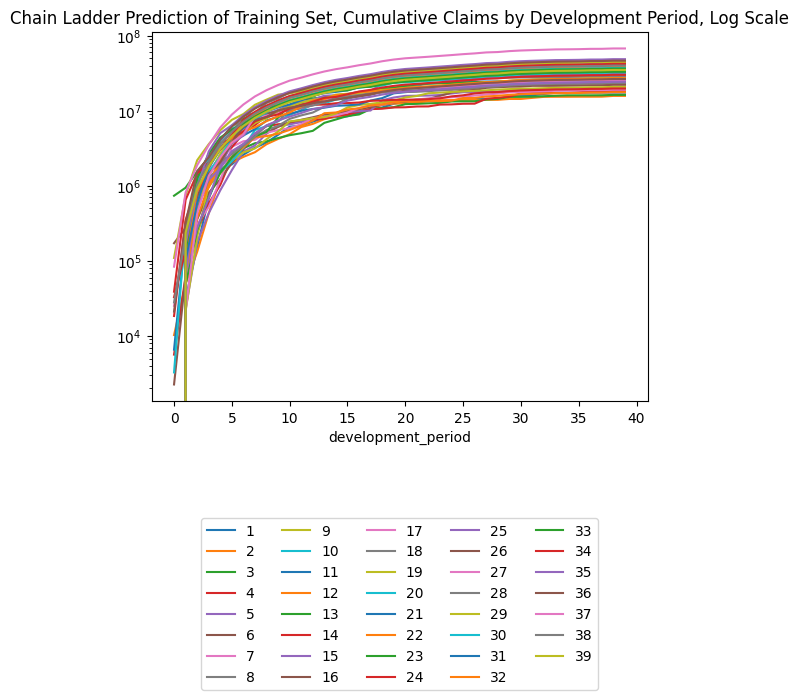

# MSE / 10^12
# Exclude occurrence period == 40 since there's no data there at cutoff
np.sum((
    triangle_cl.loc[lambda df: df.occurrence_period != cutoff].payment_size_cumulative.values - 
    triangle.loc[lambda df: df.occurrence_period != cutoff].payment_size_cumulative.values
)**2)/10**12

27656.166297305088

Chain Ladder, GLM, Aggregated Data

Chain ladders can be replicated with a GLM as discussed in our earlier article. To do this use:

• Quasipoisson distribution was used in the article (here just Poisson)
• Log Link
• Incremental ~ 0 + accident_period_factor + development_period_factor. I.e. No intercept. One factor per accident and development period.

Here we will use Torch, a package for neural networks, initially to do a GLM. Idea being that if it works, one could then test deep learning components to it. * Poisson loss * Log Link * Incremental ~ accident_period_factor + development_period_factor, but with intercept (seems to converge better this way)

Doing this at the claim level should give similar results just divided by number of claims.

class LogLinkGLM(nn.Module):
    # Define the parameters in __init__
    def __init__(
        self, 
        n_input,         # number of inputs
        n_output,        # number of outputs
        init_bias,       # init mean value to speed up convergence
        has_bias=True,   # use bias (intercept) or not       
        **kwargs,        # Ignored; Not used
    ):
        super(LogLinkGLM, self).__init__()
        
        self.linear = torch.nn.Linear(n_input, n_output, has_bias)  # Linear coefficients
        nn.init.zeros_(self.linear.weight)                          # Initialise to zero
        if has_bias:    
            self.linear.bias.data = torch.tensor(init_bias)


    # The forward functions defines how you get y from X.
    def forward(self, x):
        return torch.exp(self.linear(x))  # log(Y) = XB -> Y = exp(XB)

# Small dataset, so we can do a high number of iterations to converge to the mechanical chain ladder figures more precisely
GLM_CL_agg = Pipeline(
    steps=[
        ("keep", ColumnKeeper(["occurrence_period", "development_period"])), 
        ('one_hot', OneHotEncoder(sparse_output=False)),       # OneHot to get one factor per
        ("model", TabularNetRegressor(LogLinkGLM, has_bias=True, max_iter=10000, max_lr=0.10))
    ]
)
GLM_CL_agg.fit(
    triangle_train,
    triangle_train.loc[:, ["payment_size"]]
)

Train RMSE:  685304.6875  Train Loss:  -9891084.0
Train RMSE:  484032.34375  Train Loss:  -10054772.0
Train RMSE:  484031.5625  Train Loss:  -10054813.0
Train RMSE:  484031.4375  Train Loss:  -10054817.0
Train RMSE:  484031.34375  Train Loss:  -10054817.0
Train RMSE:  484031.375  Train Loss:  -10054817.0
Train RMSE:  484031.40625  Train Loss:  -10054817.0
Train RMSE:  484031.375  Train Loss:  -10054818.0
Train RMSE:  484031.375  Train Loss:  -10054817.0
Train RMSE:  484031.375  Train Loss:  -10054818.0

Pipeline(steps=[('keep',
                 ColumnKeeper(cols=['occurrence_period',
                                    'development_period'])),
                ('one_hot', OneHotEncoder(sparse_output=False)),
                ('model',
                 TabularNetRegressor(max_iter=10000, max_lr=0.1,
                                     module=<class '__main__.LogLinkGLM'>))])

In a Jupyter environment, please rerun this cell to show the HTML representation or trust the notebook.
On GitHub, the HTML representation is unable to render, please try loading this page with nbviewer.org.

triangle_train

	occurrence_period	development_period	payment_period	payment_size_cumulative	payment_size
0	1	0	1	0.00	0.00
1	1	1	2	31,551.25	31,551.25
2	1	2	3	152,793.12	121,241.88
3	1	3	4	680,415.06	527,621.94
4	1	4	5	1,650,518.75	970,103.75
...	...	...	...	...	...
1481	38	1	39	216,292.89	188,254.41
1482	38	2	40	1,041,738.56	825,445.62
1520	39	0	39	0.00	0.00
1521	39	1	40	237,799.91	237,799.91
1560	40	0	40	0.00	0.00

820 rows × 5 columns

triangle_glm_agg = pd.concat(
    [
        triangle_train,
        triangle_test.assign(payment_size = GLM_CL_agg.predict(triangle_test))
    ], 
    axis="rows"
).sort_values(by=["occurrence_period", "development_period"])

triangle_glm_agg["payment_size_cumulative"] = (
    triangle_glm_agg[["occurrence_period", "payment_size"]].groupby('occurrence_period').cumsum()
)
triangle_glm_agg.pivot(index = "occurrence_period", columns = "development_period", values = "payment_size_cumulative")

development_period	0	1	2	3	4	5	6	7	8	9	...	30	31	32	33	34	35	36	37	38	39
occurrence_period
1	0.00	31,551.25	152,793.14	680,415.06	1,650,518.75	1,932,605.62	2,602,592.25	3,222,089.50	3,775,028.25	4,788,738.50	...	15,739,832.00	16,082,119.00	16,780,244.00	17,400,658.00	17,422,826.00	17,422,826.00	17,485,892.00	17,485,892.00	17,485,892.00	17,485,892.00
2	10,286.75	49,493.38	132,020.67	430,670.75	1,225,081.75	2,044,801.25	2,433,025.00	2,808,325.75	3,586,153.00	4,218,801.50	...	14,386,516.00	14,880,894.00	15,342,595.00	15,378,178.00	15,378,178.00	15,409,743.00	15,409,743.00	15,433,019.00	15,795,103.00	15,795,134.00
3	0.00	62,389.38	640,980.81	987,639.94	1,536,782.25	2,385,404.00	3,177,442.25	3,698,036.50	3,918,063.50	4,333,062.00	...	15,336,449.00	15,437,039.00	15,646,281.00	15,867,258.00	16,067,564.00	16,067,564.00	16,071,147.00	16,108,434.00	16,285,614.00	16,285,647.00
4	5,646.32	63,203.44	245,984.02	584,083.56	1,030,191.25	2,371,411.75	3,179,435.75	4,964,554.00	6,244,163.00	6,612,675.00	...	17,058,208.00	17,107,564.00	17,202,888.00	17,256,650.00	17,256,650.00	17,598,124.00	18,155,534.00	18,177,990.00	18,377,934.00	18,377,972.00
5	0.00	22,911.55	177,779.52	431,647.50	872,806.00	1,619,887.12	2,862,273.00	3,462,464.75	4,956,769.00	6,237,362.50	...	19,066,432.00	19,121,176.00	19,157,450.00	19,222,536.00	19,222,536.00	19,235,524.00	19,416,042.00	19,440,056.00	19,653,882.00	19,653,922.00
6	2,259.24	62,889.90	357,107.84	813,191.12	1,218,815.75	2,030,866.75	3,065,646.00	4,652,615.50	5,097,719.50	6,097,211.00	...	21,011,932.00	21,511,248.00	21,511,248.00	21,511,248.00	21,611,440.00	21,709,188.00	21,912,920.00	21,940,022.00	22,181,346.00	22,181,390.00
7	25,200.05	212,996.06	303,872.44	522,915.66	1,180,820.75	3,314,907.25	3,931,794.50	4,110,920.00	5,112,089.00	5,522,927.00	...	17,723,798.00	18,120,490.00	18,120,490.00	18,526,526.00	18,582,586.00	18,666,634.00	18,841,812.00	18,865,116.00	19,072,620.00	19,072,656.00
8	0.00	101,324.27	482,201.94	1,302,672.88	1,762,479.38	2,816,009.75	3,599,199.00	4,404,539.50	5,549,806.50	6,296,549.50	...	27,771,816.00	27,771,816.00	27,839,500.00	28,154,842.00	28,240,034.00	28,367,762.00	28,633,984.00	28,669,398.00	28,984,740.00	28,984,798.00
9	0.00	21,563.11	207,902.11	1,019,339.94	1,467,485.12	2,183,192.50	2,792,763.75	3,155,922.75	4,188,714.25	5,294,733.50	...	19,726,482.00	19,798,286.00	20,005,244.00	20,231,846.00	20,293,066.00	20,384,850.00	20,576,154.00	20,601,604.00	20,828,206.00	20,828,248.00
10	0.00	62,438.00	642,477.19	1,220,444.00	1,512,127.75	2,125,861.00	3,205,997.50	5,542,220.00	6,233,909.00	7,278,580.50	...	23,628,224.00	23,911,102.00	24,161,056.00	24,434,730.00	24,508,666.00	24,619,518.00	24,850,564.00	24,881,298.00	25,154,974.00	25,155,024.00
11	6,573.56	233,421.70	858,658.44	1,487,226.75	2,326,138.75	4,001,959.50	4,689,719.00	5,703,576.50	7,421,133.00	8,338,611.50	...	25,062,908.00	25,362,962.00	25,628,092.00	25,918,384.00	25,996,808.00	26,114,392.00	26,359,466.00	26,392,068.00	26,682,360.00	26,682,414.00
12	0.00	337,785.12	602,649.94	947,861.81	1,960,324.25	2,438,331.25	3,263,283.25	4,443,729.00	4,600,126.00	4,950,643.00	...	16,612,003.00	16,810,882.00	16,986,614.00	17,179,024.00	17,231,004.00	17,308,940.00	17,471,378.00	17,492,986.00	17,685,396.00	17,685,432.00
13	0.00	48,432.94	257,028.44	713,263.12	1,489,202.25	2,399,702.50	3,479,596.50	4,570,094.00	5,228,066.00	8,120,785.50	...	25,494,660.00	25,799,882.00	26,069,580.00	26,364,872.00	26,444,650.00	26,564,258.00	26,813,552.00	26,846,716.00	27,142,010.00	27,142,064.00
14	18,463.75	352,189.09	1,015,863.62	1,451,495.75	2,553,104.50	3,266,427.50	5,020,334.50	6,462,674.50	8,515,544.00	9,761,135.00	...	18,626,318.00	18,849,314.00	19,046,354.00	19,262,094.00	19,320,378.00	19,407,764.00	19,589,898.00	19,614,128.00	19,829,868.00	19,829,908.00
15	0.00	64,434.53	272,821.25	689,155.88	1,832,749.12	3,660,129.75	4,680,136.50	7,358,847.00	9,028,388.00	10,283,630.00	...	29,044,080.00	29,391,798.00	29,699,042.00	30,035,448.00	30,126,330.00	30,262,590.00	30,546,594.00	30,584,374.00	30,920,780.00	30,920,842.00
16	172,118.23	276,003.81	1,468,529.00	2,473,900.50	3,320,296.00	4,172,269.00	6,421,418.50	7,663,898.50	9,201,556.00	9,852,889.00	...	22,027,450.00	22,291,162.00	22,524,182.00	22,779,316.00	22,848,242.00	22,951,584.00	23,166,976.00	23,195,630.00	23,450,764.00	23,450,812.00
17	0.00	115,323.28	533,563.88	1,628,512.75	3,782,490.00	5,496,876.00	7,221,503.00	8,019,986.00	8,644,119.00	9,252,501.00	...	24,161,342.00	24,450,602.00	24,706,194.00	24,986,044.00	25,061,650.00	25,175,002.00	25,411,260.00	25,442,690.00	25,722,540.00	25,722,592.00
18	0.00	113,693.24	534,180.81	1,126,199.38	2,086,124.25	2,636,258.50	3,415,784.25	4,550,892.50	6,384,181.50	7,276,585.00	...	22,122,974.00	22,387,832.00	22,621,862.00	22,878,102.00	22,947,328.00	23,051,118.00	23,267,444.00	23,296,222.00	23,552,462.00	23,552,510.00
19	0.00	65,176.80	593,353.38	1,377,092.75	2,679,311.00	4,561,606.50	5,190,826.50	6,896,303.00	7,889,414.50	10,040,150.00	...	25,454,734.00	25,759,478.00	26,028,754.00	26,323,584.00	26,403,236.00	26,522,656.00	26,771,562.00	26,804,674.00	27,099,504.00	27,099,558.00
20	3,269.31	303,522.59	789,422.50	1,556,370.62	2,431,901.50	4,251,400.00	6,718,960.50	9,005,604.00	10,659,464.00	12,031,561.00	...	30,440,730.00	30,805,166.00	31,127,186.00	31,479,768.00	31,575,020.00	31,717,834.00	32,015,494.00	32,055,090.00	32,407,674.00	32,407,738.00
21	0.00	99,668.09	1,164,366.00	1,829,524.50	3,262,251.75	4,136,418.00	5,829,693.00	7,624,765.00	9,753,254.00	11,093,190.00	...	31,515,314.00	31,892,618.00	32,226,004.00	32,591,032.00	32,689,648.00	32,837,502.00	33,145,670.00	33,186,666.00	33,551,694.00	33,551,760.00
22	0.00	73,295.09	370,612.00	1,025,605.62	2,284,124.00	3,889,548.50	5,347,188.00	6,029,389.00	7,281,125.00	8,422,002.00	...	25,589,258.00	25,895,614.00	26,166,310.00	26,462,700.00	26,542,772.00	26,662,824.00	26,913,044.00	26,946,332.00	27,242,722.00	27,242,776.00
23	738,959.81	944,850.44	1,558,499.75	2,354,515.50	4,080,220.25	6,339,416.00	7,833,012.00	9,289,169.00	11,375,192.00	12,184,491.00	...	31,142,902.00	31,515,746.00	31,845,194.00	32,205,908.00	32,303,358.00	32,449,466.00	32,753,990.00	32,794,502.00	33,155,218.00	33,155,284.00
24	32,878.80	139,590.50	722,637.12	2,000,021.75	3,699,119.00	4,275,938.00	5,317,856.00	7,233,628.00	8,291,626.50	8,943,028.00	...	28,343,994.00	28,683,330.00	28,983,168.00	29,311,464.00	29,400,156.00	29,533,132.00	29,810,290.00	29,847,160.00	30,175,456.00	30,175,516.00
25	0.00	67,300.14	794,740.44	1,203,488.25	1,704,533.00	2,902,497.50	3,623,180.75	4,985,555.50	6,397,038.50	7,434,320.50	...	22,882,390.00	23,156,338.00	23,398,400.00	23,663,438.00	23,735,040.00	23,842,392.00	24,066,144.00	24,095,910.00	24,360,948.00	24,360,996.00
26	0.00	222,579.27	724,894.44	1,461,998.50	2,063,614.62	3,727,648.00	6,192,158.00	7,523,791.00	8,246,266.00	10,140,250.00	...	24,910,632.00	25,208,862.00	25,472,382.00	25,760,910.00	25,838,858.00	25,955,728.00	26,199,312.00	26,231,716.00	26,520,246.00	26,520,298.00
27	0.00	21,265.95	431,409.00	1,352,109.50	2,414,385.00	3,756,162.50	4,874,574.00	8,397,044.00	10,588,448.00	11,796,448.00	...	36,532,016.00	36,969,380.00	37,355,836.00	37,778,968.00	37,893,284.00	38,064,672.00	38,421,896.00	38,469,416.00	38,892,552.00	38,892,628.00
28	0.00	281,462.16	1,313,574.88	2,223,132.00	3,606,104.50	5,205,782.00	8,583,559.00	9,386,136.00	12,726,494.00	14,633,823.00	...	42,857,548.00	43,370,640.00	43,824,008.00	44,320,408.00	44,454,516.00	44,655,584.00	45,074,660.00	45,130,408.00	45,626,808.00	45,626,900.00
29	109,492.41	749,180.50	2,196,492.25	3,589,296.50	5,510,728.00	7,582,901.50	9,060,910.00	12,036,241.00	14,089,931.00	16,412,483.00	...	41,941,452.00	42,443,580.00	42,887,260.00	43,373,048.00	43,504,288.00	43,701,056.00	44,111,176.00	44,165,732.00	44,651,524.00	44,651,612.00
30	0.00	152,130.56	1,171,098.38	2,392,989.50	4,038,955.50	5,796,676.00	6,487,593.00	7,935,940.00	9,448,145.00	12,658,112.00	...	35,222,176.00	35,643,860.00	36,016,460.00	36,424,424.00	36,534,636.00	36,699,884.00	37,044,296.00	37,090,116.00	37,498,076.00	37,498,152.00
31	0.00	102,149.25	587,694.50	1,739,223.50	3,054,168.25	4,391,554.00	6,488,115.50	8,532,481.00	9,589,075.00	13,596,397.00	...	39,249,012.00	39,718,904.00	40,134,100.00	40,588,704.00	40,711,520.00	40,895,656.00	41,279,448.00	41,330,504.00	41,785,108.00	41,785,192.00
32	0.00	137,841.00	841,636.31	1,810,914.25	3,203,533.50	4,339,657.00	7,193,541.50	8,792,350.00	11,048,168.00	12,931,037.00	...	37,328,300.00	37,775,196.00	38,170,076.00	38,602,432.00	38,719,236.00	38,894,364.00	39,259,372.00	39,307,928.00	39,740,288.00	39,740,368.00
33	0.00	134,954.59	1,254,893.38	2,674,034.25	4,403,876.00	5,591,899.50	6,810,711.50	8,387,086.00	10,152,019.00	11,882,161.00	...	34,300,500.00	34,711,148.00	35,074,000.00	35,471,288.00	35,578,616.00	35,739,540.00	36,074,940.00	36,119,560.00	36,516,848.00	36,516,920.00
34	38,893.38	652,741.81	1,456,564.38	2,050,356.00	3,044,004.00	4,796,483.00	7,570,764.00	9,698,433.00	11,739,319.00	13,739,974.00	...	39,663,492.00	40,138,348.00	40,557,928.00	41,017,336.00	41,141,448.00	41,327,528.00	41,715,372.00	41,766,968.00	42,226,372.00	42,226,456.00
35	0.00	167,482.09	926,322.88	2,872,798.50	5,040,902.00	6,421,425.50	8,743,438.00	11,200,672.00	13,557,681.00	15,868,229.00	...	45,807,164.00	46,355,568.00	46,840,140.00	47,370,704.00	47,514,044.00	47,728,948.00	48,176,864.00	48,236,452.00	48,767,016.00	48,767,112.00
36	21,154.29	320,832.62	1,568,433.12	2,393,324.00	4,121,508.50	6,130,129.00	8,346,808.00	10,692,576.00	12,942,664.00	15,148,399.00	...	43,729,208.00	44,252,736.00	44,715,328.00	45,221,824.00	45,358,660.00	45,563,816.00	45,991,416.00	46,048,296.00	46,554,796.00	46,554,888.00
37	83,818.48	819,248.56	1,881,916.25	3,489,761.75	5,992,953.00	8,913,622.00	12,136,824.00	15,547,728.00	18,819,508.00	22,026,796.00	...	63,585,224.00	64,346,468.00	65,019,108.00	65,755,588.00	65,954,552.00	66,252,864.00	66,874,624.00	66,957,336.00	67,693,816.00	67,693,952.00
38	28,038.49	216,292.89	1,041,738.50	2,063,425.25	3,543,510.50	5,270,441.50	7,176,253.50	9,193,051.00	11,127,587.00	13,023,989.00	...	37,596,636.00	38,046,744.00	38,444,464.00	38,879,928.00	38,997,576.00	39,173,960.00	39,541,592.00	39,590,500.00	40,025,964.00	40,026,044.00
39	0.00	237,799.91	910,953.75	1,804,373.88	3,098,643.00	4,608,768.00	6,275,317.00	8,038,917.00	9,730,584.00	11,388,904.00	...	32,876,592.00	33,270,192.00	33,617,980.00	33,998,776.00	34,101,648.00	34,255,892.00	34,577,368.00	34,620,136.00	35,000,932.00	35,001,000.00
40	0.00	166.40	726.71	1,470.36	2,547.66	3,804.63	5,191.81	6,659.76	8,067.84	9,448.17	...	27,333.73	27,661.35	27,950.83	28,267.79	28,353.42	28,481.80	28,749.39	28,784.99	29,101.95	29,102.01

40 rows × 40 columns

Check difference with chain ladder. These seem quite small, except for occurrence period 40 where our log link is unable to get the value to zero.

(triangle_glm_agg.pivot(index = "occurrence_period", columns = "development_period", values = "payment_size_cumulative") - 
triangle_cl.pivot(index = "occurrence_period", columns = "development_period", values = "payment_size_cumulative"))

development_period	0	1	2	3	4	5	6	7	8	9	...	30	31	32	33	34	35	36	37	38	39
occurrence_period
1	0.00	0.00	0.02	0.00	0.00	0.00	0.00	0.00	0.00	0.00	...	0.00	0.00	-2.00	0.00	0.00	0.00	0.00	0.00	0.00	0.00
2	0.00	0.00	0.00	0.00	0.00	0.12	0.00	0.00	0.00	0.00	...	0.00	0.00	0.00	0.00	0.00	0.00	0.00	0.00	0.00	31.00
3	0.00	0.00	0.00	-0.06	0.00	0.00	0.00	0.00	0.00	0.00	...	0.00	0.00	0.00	0.00	0.00	0.00	0.00	0.00	-2.00	31.00
4	0.00	0.00	-0.02	-0.06	-0.06	0.00	0.00	0.00	0.00	0.00	...	0.00	0.00	0.00	0.00	0.00	0.00	0.00	2.00	0.00	38.00
5	0.00	0.00	0.00	0.00	0.06	0.12	0.00	0.00	-0.50	0.00	...	-2.00	-2.00	0.00	-2.00	-2.00	0.00	-2.00	-2.00	-4.00	36.00
6	0.00	-0.00	0.00	0.00	0.00	-0.12	0.00	0.00	0.00	0.00	...	0.00	0.00	0.00	0.00	0.00	2.00	-2.00	-2.00	-4.00	40.00
7	0.00	0.00	0.00	0.00	-0.12	0.00	0.25	0.00	0.00	0.00	...	0.00	0.00	0.00	0.00	0.00	0.00	-4.00	-4.00	-4.00	32.00
8	0.00	0.00	0.00	0.00	0.00	0.00	0.00	0.00	0.00	0.00	...	0.00	0.00	0.00	0.00	-2.00	-2.00	-4.00	-4.00	-6.00	52.00
9	0.00	0.00	0.00	0.00	0.00	0.00	0.00	0.00	0.00	0.00	...	-2.00	0.00	-2.00	-2.00	-2.00	-2.00	-4.00	-2.00	-4.00	38.00
10	0.00	0.00	0.00	0.12	0.00	0.25	0.25	0.00	-0.50	-0.50	...	0.00	0.00	0.00	-2.00	-2.00	0.00	-2.00	-4.00	-6.00	44.00
11	0.00	0.00	0.06	0.00	0.00	0.00	0.00	0.00	0.00	0.00	...	0.00	0.00	0.00	-2.00	-4.00	-2.00	-6.00	-6.00	-8.00	46.00
12	0.00	0.00	0.00	0.00	-0.12	0.00	0.00	0.00	0.00	0.00	...	-2.00	-4.00	-4.00	-4.00	-6.00	-4.00	-6.00	-6.00	-8.00	28.00
13	0.00	0.00	0.00	0.00	0.00	0.00	-0.25	0.00	0.00	0.00	...	-2.00	-4.00	-4.00	-6.00	-6.00	-6.00	-12.00	-10.00	-12.00	42.00
14	0.00	0.00	0.00	0.00	0.25	0.00	0.50	0.50	0.00	1.00	...	-2.00	-2.00	-2.00	-2.00	-2.00	0.00	-4.00	-2.00	-4.00	36.00
15	0.00	0.00	0.00	0.00	0.00	0.00	0.00	0.00	0.00	1.00	...	0.00	0.00	-2.00	-2.00	-4.00	-2.00	-4.00	-4.00	-6.00	56.00
16	0.00	0.00	0.00	0.00	-0.25	-0.25	0.00	0.00	0.00	0.00	...	2.00	0.00	0.00	0.00	-2.00	0.00	-2.00	0.00	-2.00	46.00
17	0.00	0.00	0.00	0.00	0.00	0.00	0.00	0.00	0.00	0.00	...	2.00	0.00	-2.00	-2.00	-2.00	-2.00	-6.00	-4.00	-6.00	46.00
18	0.00	0.00	0.00	0.00	0.12	0.00	0.00	0.00	0.00	0.00	...	0.00	0.00	0.00	-2.00	-2.00	0.00	-4.00	-4.00	-6.00	42.00
19	0.00	0.00	0.00	0.00	-0.25	0.00	0.00	0.50	0.00	0.00	...	2.00	0.00	0.00	-2.00	-2.00	-2.00	-4.00	-2.00	-6.00	48.00
20	0.00	0.00	0.00	0.12	0.00	0.00	0.00	-1.00	0.00	0.00	...	2.00	0.00	0.00	0.00	-2.00	0.00	-4.00	-4.00	-4.00	60.00
21	0.00	0.00	0.00	0.12	0.25	0.25	0.00	0.00	-1.00	0.00	...	4.00	4.00	2.00	2.00	2.00	4.00	0.00	2.00	0.00	66.00
22	0.00	0.00	0.00	0.06	0.00	-0.25	0.00	0.00	0.50	0.00	...	8.00	8.00	6.00	6.00	4.00	6.00	2.00	4.00	2.00	56.00
23	0.00	0.00	-0.12	0.00	0.00	0.00	0.00	0.00	0.00	0.00	...	6.00	6.00	6.00	4.00	2.00	4.00	-2.00	0.00	-2.00	64.00
24	0.00	0.00	0.00	0.00	0.00	-0.50	0.00	0.50	0.00	0.00	...	4.00	4.00	2.00	2.00	0.00	2.00	-2.00	-2.00	-4.00	56.00
25	0.00	0.00	0.00	0.00	0.00	0.25	0.00	0.00	0.00	0.00	...	2.00	0.00	-2.00	-2.00	-2.00	-2.00	-4.00	-2.00	-2.00	46.00
26	0.00	0.00	0.00	0.00	0.00	0.00	0.00	0.50	0.50	0.00	...	4.00	2.00	2.00	0.00	-2.00	0.00	-4.00	-4.00	-6.00	46.00
27	0.00	0.00	0.00	0.00	0.00	0.00	0.00	0.00	1.00	0.00	...	8.00	8.00	8.00	4.00	4.00	4.00	0.00	0.00	0.00	76.00
28	0.00	0.00	0.00	-0.25	-0.25	0.00	0.00	0.00	0.00	0.00	...	12.00	12.00	8.00	8.00	8.00	12.00	8.00	8.00	4.00	96.00
29	0.00	0.00	0.00	0.25	0.00	0.00	0.00	0.00	0.00	0.00	...	12.00	16.00	12.00	8.00	4.00	4.00	0.00	0.00	0.00	88.00
30	0.00	0.00	0.00	0.25	0.00	0.50	0.00	0.00	0.00	0.00	...	20.00	20.00	20.00	20.00	16.00	20.00	12.00	16.00	12.00	88.00
31	0.00	0.00	0.00	0.00	0.00	0.00	0.00	0.00	0.00	0.00	...	8.00	8.00	4.00	4.00	4.00	4.00	0.00	0.00	-4.00	80.00
32	0.00	0.00	0.00	0.00	0.00	0.00	0.00	0.00	0.00	1.00	...	16.00	16.00	16.00	16.00	12.00	16.00	12.00	12.00	12.00	92.00
33	0.00	0.00	0.00	0.00	0.00	0.00	0.00	0.00	-1.00	-2.00	...	16.00	16.00	16.00	16.00	12.00	16.00	8.00	12.00	8.00	80.00
34	0.00	0.00	0.00	0.00	0.00	0.00	0.00	0.00	-1.00	-2.00	...	24.00	28.00	24.00	28.00	28.00	28.00	24.00	28.00	24.00	108.00
35	0.00	0.00	0.00	0.00	0.00	0.00	0.00	-1.00	-2.00	-2.00	...	12.00	8.00	4.00	4.00	4.00	4.00	-4.00	0.00	-4.00	92.00
36	0.00	-0.03	0.00	0.00	0.00	2.00	2.50	5.00	5.00	7.00	...	36.00	36.00	36.00	36.00	36.00	40.00	36.00	36.00	36.00	128.00
37	0.00	0.00	0.00	0.00	3.50	6.00	9.00	12.00	14.00	18.00	...	72.00	72.00	68.00	68.00	64.00	68.00	60.00	60.00	56.00	192.00
38	0.00	0.00	-0.06	1.12	3.00	4.50	5.50	8.00	9.00	10.00	...	40.00	40.00	40.00	40.00	40.00	40.00	36.00	40.00	36.00	116.00
39	0.00	0.00	2.81	7.38	13.75	20.50	28.00	36.00	44.00	51.00	...	156.00	158.00	160.00	160.00	156.00	160.00	156.00	160.00	160.00	228.00
40	0.00	166.40	726.71	1,470.36	2,547.66	3,804.63	5,191.81	6,659.76	8,067.84	9,448.17	...	27,333.73	27,661.35	27,950.83	28,267.79	28,353.42	28,481.80	28,749.39	28,784.99	29,101.95	29,102.01

40 rows × 40 columns

(triangle_glm_agg
    .loc[lambda df: df.occurrence_period != cutoff]  # Exclude occurrence period == 40 since there's no data there at cutoff
    .pivot(index = "development_period", columns = "occurrence_period", values = "payment_size_cumulative")
    .plot(logy=True)
)
plt.title("GLM Chain Ladder Prediction of Training Set, Cumulative Claims by Development Period, Log Scale")
plt.legend(loc="lower center", bbox_to_anchor=(0.5, -0.8), ncol=5)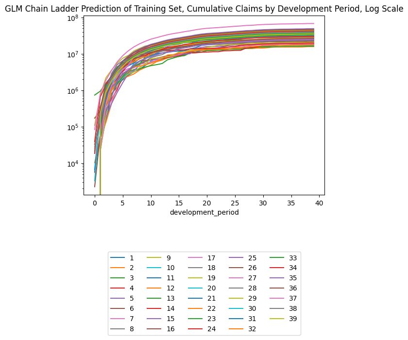

<matplotlib.legend.Legend at 0x2ac9d3910>

# MSE / 10^12
# Exclude occurrence period == 40 since there's no data there at cutoff
np.sum((
    triangle_glm_agg.loc[lambda df: df.occurrence_period != cutoff].payment_size_cumulative.values - 
    triangle.loc[lambda df: df.occurrence_period != cutoff].payment_size_cumulative.values
)**2)/10**12

27656.19636207616

GLM, Occurrence/Development Only, Individual Data

What if we just fit the same “chain ladder” model on the individual data?

One limitation moving to individual data, is that we would be predicting ultimates including claims that we would not be normally aware of yet. This is, however, a limitation with most individual claims models. A method of overcoming this could be to start at the policy rather than at the claim (and following this same process of one record per period), however our dataset is at the claim level.

GLM_CL_ind = Pipeline(
    steps=[
        ("keep", ColumnKeeper(["occurrence_period", "development_period"])), 
        ('one_hot', OneHotEncoder(sparse_output=False)),       # OneHot to get one factor per
        ("model", TabularNetRegressor(LogLinkGLM, has_bias=True, max_iter=glm_iter, max_lr=0.05))
    ]
)
GLM_CL_ind.fit(
    dat.loc[dat.train_ind == 1],
    dat.loc[dat.train_ind, ["payment_size"]]
)

Train RMSE:  55491.80859375  Train Loss:  -76383.375
Train RMSE:  55302.078125  Train Loss:  -77458.4453125
Train RMSE:  55260.9375  Train Loss:  -77752.9296875
Train RMSE:  55260.1640625  Train Loss:  -77769.5703125
Train RMSE:  55260.1015625  Train Loss:  -77773.015625
Train RMSE:  55260.0859375  Train Loss:  -77774.140625
Train RMSE:  55260.08203125  Train Loss:  -77774.5859375
Train RMSE:  55260.078125  Train Loss:  -77774.7890625
Train RMSE:  55260.078125  Train Loss:  -77774.8828125
Train RMSE:  55260.08203125  Train Loss:  -77774.9140625

Pipeline(steps=[('keep',
                 ColumnKeeper(cols=['occurrence_period',
                                    'development_period'])),
                ('one_hot', OneHotEncoder(sparse_output=False)),
                ('model',
                 TabularNetRegressor(max_iter=500, max_lr=0.05,
                                     module=<class '__main__.LogLinkGLM'>))])

In a Jupyter environment, please rerun this cell to show the HTML representation or trust the notebook.
On GitHub, the HTML representation is unable to render, please try loading this page with nbviewer.org.

# Function to make a dataset with train payments and test predictions, and resulting triangle
def make_pred_set_and_triangle(individual_model, train, test):
    dat_model_pred = pd.concat(
        [
            train,
            test.assign(payment_size = individual_model.predict(test))
        ], 
        axis="rows"
    )
    dat_model_pred["payment_size_cumulative"] = (
        dat_model_pred[["claim_no", "payment_size"]].groupby('claim_no').cumsum()
    )

    triangle_model_ind = (dat_model_pred
        .groupby(["occurrence_period", "development_period", "payment_period"], as_index=False)
        .agg({"payment_size_cumulative": "sum", "payment_size": "sum"})
        .sort_values(by=["occurrence_period", "development_period"])
    )

    (triangle_model_ind
        .loc[lambda df: (df.occurrence_period != cutoff) & (df.development_period < cutoff)]
        .pivot(index = "development_period", columns = "occurrence_period", values = "payment_size_cumulative")
        .plot(logy=True)
    )
    plt.legend(loc="lower center", bbox_to_anchor=(0.5, -0.8), ncol=5)
    plt.title("Cumulative Claims by Development - Predictions Lower Half Triangle")

    return dat_model_pred, triangle_model_ind

dat_glm_pred, triangle_glm_ind = make_pred_set_and_triangle(GLM_CL_ind, dat.loc[dat.train_ind == 1], dat.loc[dat.train_ind == 0])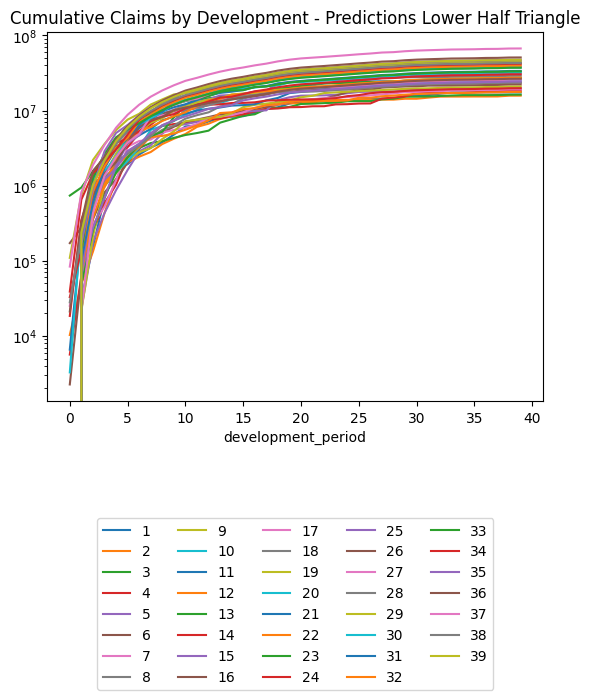

Looks to be giving a reasonable curve.

Differences with Chain Ladder

Differences in GLM coefficients with aggregated data:

start = cutoff
end = cutoff + num_dev_periods + 1
start, end

(40, 80)

GLM_CL_agg["model"].module_.linear.weight.data[: ,start:end].cpu().numpy().ravel()

array([-2.6085851 , -0.9452279 ,  0.26885098,  0.55193317,  0.92257833,
        1.0768248 ,  1.175387  ,  1.2319895 ,  1.1903464 ,  1.1704375 ,
        1.1738193 ,  0.88819265,  1.0728831 ,  1.0463339 ,  0.9118993 ,
        0.7312811 ,  0.9362656 ,  0.8054807 ,  1.1134231 ,  0.89804524,
        0.63513625,  0.19344859,  0.19643542,  0.3392283 ,  0.33730403,
        0.45425934,  0.2924858 ,  0.5794589 , -0.3311628 ,  0.55835927,
        0.17237537, -0.26778826, -0.39153227, -0.30086178, -1.6096059 ,
       -1.2046075 , -0.47019288, -2.487373  , -0.30085984, -8.907836  ],
      dtype=float32)

GLM_CL_ind["model"].module_.linear.weight.data[: ,start:end].cpu().numpy().ravel()

array([-0.95821226, -0.6363852 ,  0.12603194,  0.20968342,  0.48075658,
        0.5889297 ,  0.6586112 ,  0.7034973 ,  0.6573421 ,  0.6352269 ,
        0.6381907 ,  0.35272628,  0.5351275 ,  0.5085579 ,  0.37453473,
        0.1936421 ,  0.3985621 ,  0.268308  ,  0.57655615,  0.361657  ,
        0.0992958 , -0.34339836, -0.34055626, -0.19771653, -0.19970702,
       -0.08316672, -0.24393895,  0.04285933, -0.86934584,  0.0212998 ,
       -0.36557752, -0.806808  , -0.9307192 , -0.83957726, -2.048075  ,
       -1.721573  , -1.0065743 , -2.4330187 , -0.8382782 , -2.7173047 ],
      dtype=float32)

pd.DataFrame.from_dict({
    "aggregate": GLM_CL_agg["model"].module_.linear.weight.data[: ,start:end].cpu().numpy().ravel(),
    "individual": GLM_CL_ind["model"].module_.linear.weight.data[: ,start:end].cpu().numpy().ravel(),
    "log_incr_perc_ultimate_shifted": np.log(df_cdf.incr_perc_of_ultimate * num_dev_periods)
}).plot()

/Users/jacky/GitRepos/NNs-on-Individual-Claims/.conda/lib/python3.10/site-packages/pandas/core/arraylike.py:402: RuntimeWarning: divide by zero encountered in log
  result = getattr(ufunc, method)(*inputs, **kwargs)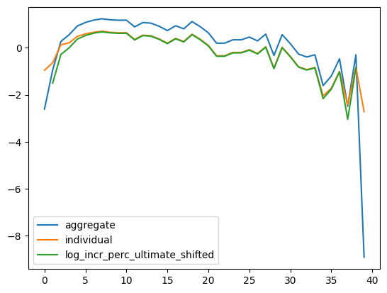

<AxesSubplot: >

Difference in predictions in direct calculation:

(triangle_glm_ind.pivot(index = "occurrence_period", columns = "development_period", values = "payment_size_cumulative") - 
triangle_cl.pivot(index = "occurrence_period", columns = "development_period", values = "payment_size_cumulative"))

development_period	0	1	2	3	4	5	6	7	8	9	...	30	31	32	33	34	35	36	37	38	39
occurrence_period
1	0.00	0.00	0.02	0.00	0.00	0.00	0.00	0.25	0.00	0.00	...	0.00	0.00	0.00	0.00	0.00	0.00	0.00	0.00	0.00	0.00
2	0.00	0.00	0.00	0.03	0.00	0.12	0.00	0.00	0.00	0.00	...	0.00	0.00	0.00	0.00	0.00	0.00	0.00	1.00	0.00	26,118.00
3	0.00	0.00	0.00	0.00	0.00	0.00	0.00	0.00	0.00	0.00	...	0.00	0.00	0.00	0.00	0.00	0.00	0.00	0.00	-541.00	26,439.00
4	0.00	-0.00	0.00	0.00	0.00	0.00	0.00	0.00	0.00	0.00	...	0.00	0.00	0.00	0.00	0.00	0.00	0.00	17,844.00	16,446.00	46,772.00
5	0.00	0.00	0.00	0.00	0.00	0.12	0.00	0.00	0.00	0.00	...	0.00	0.00	2.00	0.00	0.00	0.00	1,940.00	21,744.00	23,818.00	56,794.00
6	0.00	0.00	0.00	0.00	0.00	0.00	0.00	0.00	0.00	0.00	...	0.00	0.00	0.00	0.00	0.00	1,718.00	1,304.00	23,032.00	22,294.00	59,042.00
7	0.00	0.00	0.00	0.00	0.00	0.00	0.00	-0.25	-0.50	0.00	...	0.00	0.00	0.00	0.00	5,974.00	7,912.00	8,500.00	27,408.00	27,892.00	59,658.00
8	0.00	0.00	0.00	0.00	0.00	0.00	0.00	0.00	0.00	0.00	...	0.00	0.00	0.00	-180.00	8,748.00	11,484.00	11,950.00	40,584.00	40,812.00	89,012.00
9	0.00	0.00	0.00	0.00	0.00	0.00	0.00	0.00	0.00	0.00	...	0.00	0.00	32.00	176.00	6,672.00	8,750.00	9,316.00	29,948.00	30,384.00	65,062.00
10	0.00	0.00	0.00	0.00	0.00	0.00	0.25	0.00	0.00	0.00	...	0.00	-698.00	-1,358.00	-1,952.00	5,668.00	7,862.00	7,896.00	32,658.00	32,418.00	74,182.00
11	0.00	0.00	0.06	0.00	0.00	0.00	0.00	0.50	0.00	0.00	...	-2,130.00	-3,820.00	-5,360.00	-6,908.00	898.00	2,844.00	2,102.00	28,182.00	27,008.00	71,168.00
12	0.00	0.00	0.00	0.00	-0.12	0.00	0.00	0.00	0.00	0.00	...	-5,279.00	-6,972.00	-8,496.00	-10,074.00	-5,064.00	-4,002.00	-4,960.00	12,214.00	10,882.00	40,066.00
13	0.00	0.00	0.00	0.00	0.00	0.00	0.00	0.00	0.00	0.00	...	-1,548.00	-2,314.00	-3,036.00	-3,688.00	4,528.00	6,890.00	6,916.00	33,634.00	33,364.00	78,426.00
14	0.00	0.00	0.00	-0.12	0.25	0.00	0.00	0.00	0.00	0.00	...	-12,584.00	-14,744.00	-16,686.00	-18,710.00	-13,170.00	-12,086.00	-13,376.00	5,828.00	4,078.00	36,764.00
15	0.00	0.00	0.00	0.00	0.00	0.00	0.00	0.00	0.00	0.00	...	35,176.00	38,468.00	41,322.00	44,608.00	55,172.00	59,532.00	62,974.00	94,228.00	97,954.00	149,906.00
16	0.00	0.00	0.00	0.25	0.00	0.00	0.00	0.00	0.00	0.00	...	-23,084.00	-25,688.00	-28,028.00	-30,468.00	-23,930.00	-22,666.00	-24,230.00	-1,528.00	-3,644.00	35,004.00
17	0.00	0.00	0.00	0.00	0.00	0.00	0.00	0.00	0.00	0.00	...	-5,364.00	-6,332.00	-7,230.00	-8,078.00	-362.00	1,780.00	1,608.00	26,880.00	26,392.00	69,062.00
18	0.00	0.00	0.00	0.00	0.00	0.00	0.00	0.00	0.00	0.00	...	-10,792.00	-12,038.00	-13,176.00	-14,304.00	-7,342.00	-5,524.00	-5,974.00	17,092.00	16,296.00	55,314.00
19	0.00	0.00	0.00	0.00	0.00	0.00	0.00	0.00	0.00	0.00	...	-14,284.00	-15,752.00	-17,094.00	-18,426.00	-10,426.00	-8,348.00	-8,896.00	17,642.00	16,690.00	61,578.00
20	0.00	0.00	0.00	0.12	0.00	0.00	0.00	0.00	0.00	0.00	...	-55,784.00	-59,628.00	-63,078.00	-66,690.00	-57,724.00	-56,078.00	-58,444.00	-27,120.00	-30,280.00	23,090.00
21	0.00	0.00	0.00	0.00	0.00	0.00	0.00	0.00	0.00	0.00	...	69,346.00	71,976.00	74,242.00	76,900.00	88,090.00	92,444.00	95,408.00	129,136.00	132,270.00	188,502.00
22	0.00	0.00	0.00	0.00	0.00	0.00	-0.50	0.00	0.00	0.00	...	55,238.00	56,924.00	58,370.00	60,092.00	69,048.00	72,404.00	74,442.00	101,742.00	103,848.00	149,442.00
23	0.00	0.00	0.00	0.00	0.00	0.00	0.00	0.00	0.00	0.00	...	54,880.00	56,070.00	57,066.00	58,326.00	68,976.00	72,712.00	74,488.00	107,540.00	109,268.00	164,628.00
24	0.00	0.00	0.00	0.00	0.00	0.00	0.00	0.50	0.00	1.00	...	116,230.00	119,328.00	122,014.00	125,112.00	135,388.00	139,596.00	142,860.00	173,338.00	176,866.00	227,548.00
25	0.00	0.00	0.00	-0.12	0.00	0.00	0.00	0.00	0.00	0.00	...	-24,200.00	-25,480.00	-26,652.00	-27,812.00	-20,608.00	-18,724.00	-19,184.00	4,678.00	3,862.00	44,220.00
26	0.00	0.00	0.00	0.00	0.00	0.00	-0.50	0.00	0.00	-1.00	...	-46,666.00	-48,544.00	-50,248.00	-51,978.00	-44,276.00	-42,422.00	-43,318.00	-17,438.00	-18,798.00	25,066.00
27	0.00	0.00	0.00	-0.12	0.00	0.00	0.00	0.00	1.00	0.00	...	110,416.00	112,332.00	113,960.00	115,940.00	128,584.00	133,176.00	135,684.00	174,560.00	177,092.00	242,108.00
28	0.00	0.00	0.00	0.00	0.00	0.00	0.00	0.00	0.00	0.00	...	-2,208.00	-3,240.00	-4,228.00	-5,076.00	8,812.00	12,884.00	13,140.00	58,104.00	57,896.00	133,684.00
29	0.00	0.00	0.00	0.00	0.00	0.00	0.00	0.00	0.00	0.00	...	-747,996.00	-764,748.00	-779,632.00	-795,700.00	-786,664.00	-788,988.00	-801,632.00	-760,728.00	-776,188.00	-704,352.00
30	0.00	0.00	0.00	0.00	0.00	0.00	0.00	0.00	0.00	0.00	...	-22,220.00	-23,488.00	-24,672.00	-25,780.00	-14,488.00	-11,312.00	-11,448.00	25,420.00	24,844.00	87,068.00
31	0.00	0.00	0.00	0.00	0.00	0.00	0.00	0.00	0.00	0.00	...	375,908.00	381,800.00	386,940.00	392,784.00	407,476.00	413,948.00	419,784.00	462,300.00	468,740.00	539,160.00
32	0.00	0.00	0.00	0.00	0.00	0.00	0.00	0.00	1.00	-10,088.00	...	-182,780.00	-186,864.00	-190,536.00	-194,356.00	-183,184.00	-180,912.00	-183,300.00	-144,764.00	-148,032.00	-82,492.00
33	0.00	0.00	0.00	0.00	0.00	0.00	0.00	0.00	27,233.00	50,059.00	...	529,056.00	537,300.00	544,524.00	552,624.00	566,356.00	573,252.00	580,884.00	618,652.00	627,272.00	689,272.00
34	0.00	0.00	0.00	0.00	0.00	0.00	0.00	-2,418.00	-13,918.00	-29,573.00	...	-276,912.00	-282,420.00	-287,356.00	-292,544.00	-281,008.00	-279,064.00	-282,552.00	-241,836.00	-246,440.00	-176,972.00
35	0.00	0.00	0.00	0.00	0.00	0.00	-70,556.00	-146,515.00	-229,660.00	-291,366.00	...	-1,141,304.00	-1,157,984.00	-1,172,796.00	-1,188,772.00	-1,178,432.00	-1,180,320.00	-1,192,800.00	-1,147,804.00	-1,163,116.00	-1,084,416.00
36	0.00	0.00	0.00	0.00	0.25	85,090.00	229,827.50	384,379.00	638,293.00	881,795.00	...	3,982,064.00	4,037,648.00	4,086,680.00	4,140,624.00	4,171,164.00	4,198,008.00	4,244,652.00	4,301,668.00	4,356,340.00	4,442,052.00
37	0.00	0.00	0.00	0.00	-74,768.50	-122,564.00	-158,118.00	-235,035.00	-287,442.00	-310,780.00	...	-684,548.00	-692,960.00	-700,508.00	-708,428.00	-689,816.00	-686,528.00	-691,788.00	-626,436.00	-633,412.00	-521,992.00
38	0.00	0.00	0.00	66,269.62	262,007.75	452,814.00	603,134.50	736,867.00	882,875.00	1,021,512.00	...	2,772,288.00	2,803,356.00	2,830,736.00	2,860,940.00	2,882,360.00	2,898,740.00	2,925,152.00	2,970,880.00	3,001,680.00	3,072,900.00
39	0.00	0.00	105,522.88	372,281.00	825,593.25	1,354,328.50	1,996,585.50	2,647,787.00	3,261,998.00	3,859,120.00	...	11,545,788.00	11,685,482.00	11,808,832.00	11,944,132.00	11,995,388.00	12,054,788.00	12,170,032.00	12,232,152.00	12,368,124.00	12,447,052.00
40	0.00	11,206.78	56,149.67	110,068.73	188,510.28	280,837.16	385,106.44	496,923.50	605,015.06	710,742.38	...	2,078,335.00	2,103,333.75	2,125,419.25	2,149,612.25	2,156,837.25	2,166,852.00	2,187,324.25	2,192,240.75	2,216,465.00	2,220,165.25

40 rows × 40 columns

# MSE / 10^12
# Exclude occurrence period == 40 since there's no data there at cutoff
np.sum((
    triangle_glm_ind.loc[lambda df: df.occurrence_period != cutoff].payment_size_cumulative.values - 
    triangle.loc[lambda df: df.occurrence_period != cutoff].payment_size_cumulative.values
)**2)/10**12

24148.42140950528

GLM with Splines, Occur/Dev, Individual Data

In Grainne McGuire’s article she uses splines in the GLM model to model a parabolic trend in occurrence period. In this example data, there is also a curve with development periods. Can we do something similar?

GLM_CL_spline = Pipeline(
    steps=[
        ("keep", ColumnKeeper(["occurrence_period", "development_period"])), 
        ('one_hot', SplineTransformer()),       # Spline transform
        ("model", TabularNetRegressor(LogLinkGLM, has_bias=True, max_iter=glm_iter, max_lr=0.05))
    ]
)
GLM_CL_spline.fit(
    dat.loc[dat.train_ind == 1],
    dat.loc[dat.train_ind, ["payment_size"]]
)

Train RMSE:  55492.2421875  Train Loss:  -76383.375
Train RMSE:  55338.0625  Train Loss:  -77265.875
Train RMSE:  55294.43359375  Train Loss:  -77546.9765625
Train RMSE:  55289.453125  Train Loss:  -77583.4375
Train RMSE:  55286.875  Train Loss:  -77601.484375
Train RMSE:  55285.2890625  Train Loss:  -77612.5078125
Train RMSE:  55284.37109375  Train Loss:  -77618.8984375
Train RMSE:  55283.875  Train Loss:  -77622.3984375
Train RMSE:  55283.62890625  Train Loss:  -77624.1328125
Train RMSE:  55283.5390625  Train Loss:  -77624.78125

Pipeline(steps=[('keep',
                 ColumnKeeper(cols=['occurrence_period',
                                    'development_period'])),
                ('one_hot', SplineTransformer()),
                ('model',
                 TabularNetRegressor(max_iter=500, max_lr=0.05,
                                     module=<class '__main__.LogLinkGLM'>))])

In a Jupyter environment, please rerun this cell to show the HTML representation or trust the notebook.
On GitHub, the HTML representation is unable to render, please try loading this page with nbviewer.org.

dat_spline_pred, triangle_spline_ind = make_pred_set_and_triangle(GLM_CL_spline, dat.loc[dat.train_ind == 1], dat.loc[dat.train_ind == 0])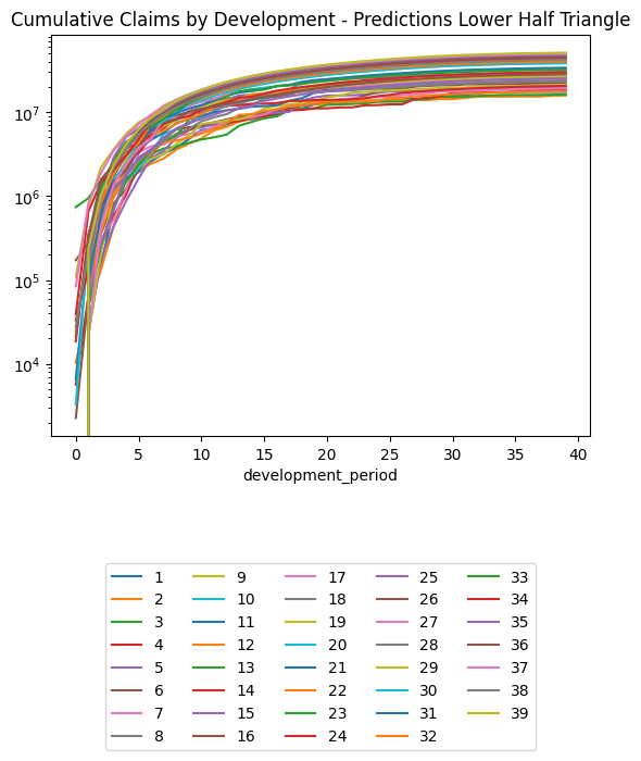

# Diagnostic model subplots
# We will be repeating this logic across multiple models, so put logic into function for repeatability

def make_model_subplots(model, dat):
    fig, axes = plt.subplots(3, 2, sharex='all', sharey='all', figsize=(15, 15))

    (dat
        .assign(payment_size_pred = model.predict(dat))
        .loc[lambda df: df.train_ind]
        .groupby(["occurrence_period"])
        .agg({"payment_size": "mean", "payment_size_pred": "mean"})
    ).plot(ax=axes[0,0], logy=True)
    axes[0,0].title.set_text("Train, Occur")

    (dat
        .assign(payment_size_pred = model.predict(dat))
        .loc[lambda df: df.train_ind]
        .groupby(["development_period"])
        .agg({"payment_size": "mean", "payment_size_pred": "mean"})
    ).plot(ax=axes[0,1], logy=True)
    axes[0,1].title.set_text("Train, Dev")

    (dat
        .assign(payment_size_pred = model.predict(dat))
        .loc[lambda df: ~df.train_ind]
        .groupby(["occurrence_period"])
        .agg({"payment_size": "mean", "payment_size_pred": "mean"})
    ).plot(ax=axes[1,0], logy=True)
    axes[1,0].title.set_text("Test, Occ")

    (dat
        .assign(payment_size_pred = model.predict(dat))
        .loc[lambda df: ~df.train_ind]
        .groupby(["development_period"])
        .agg({"payment_size": "mean", "payment_size_pred": "mean"})
    ).plot(ax=axes[1,1], logy=True)
    axes[1,1].title.set_text("Test, Dev")

    (dat
        .assign(payment_size_pred = model.predict(dat))
        .groupby(["occurrence_period"])
        .agg({"payment_size": "mean", "payment_size_pred": "mean"})
    ).plot(ax=axes[2,0], logy=True)
    axes[2,0].title.set_text("All, Occ")

    (dat
        .assign(payment_size_pred = model.predict(dat))
        .groupby(["development_period"])
        .agg({"payment_size": "mean", "payment_size_pred": "mean"})
    ).plot(ax=axes[2,1], logy=True)
    axes[2,1].title.set_text("All, Dev")

make_model_subplots(GLM_CL_spline, dat)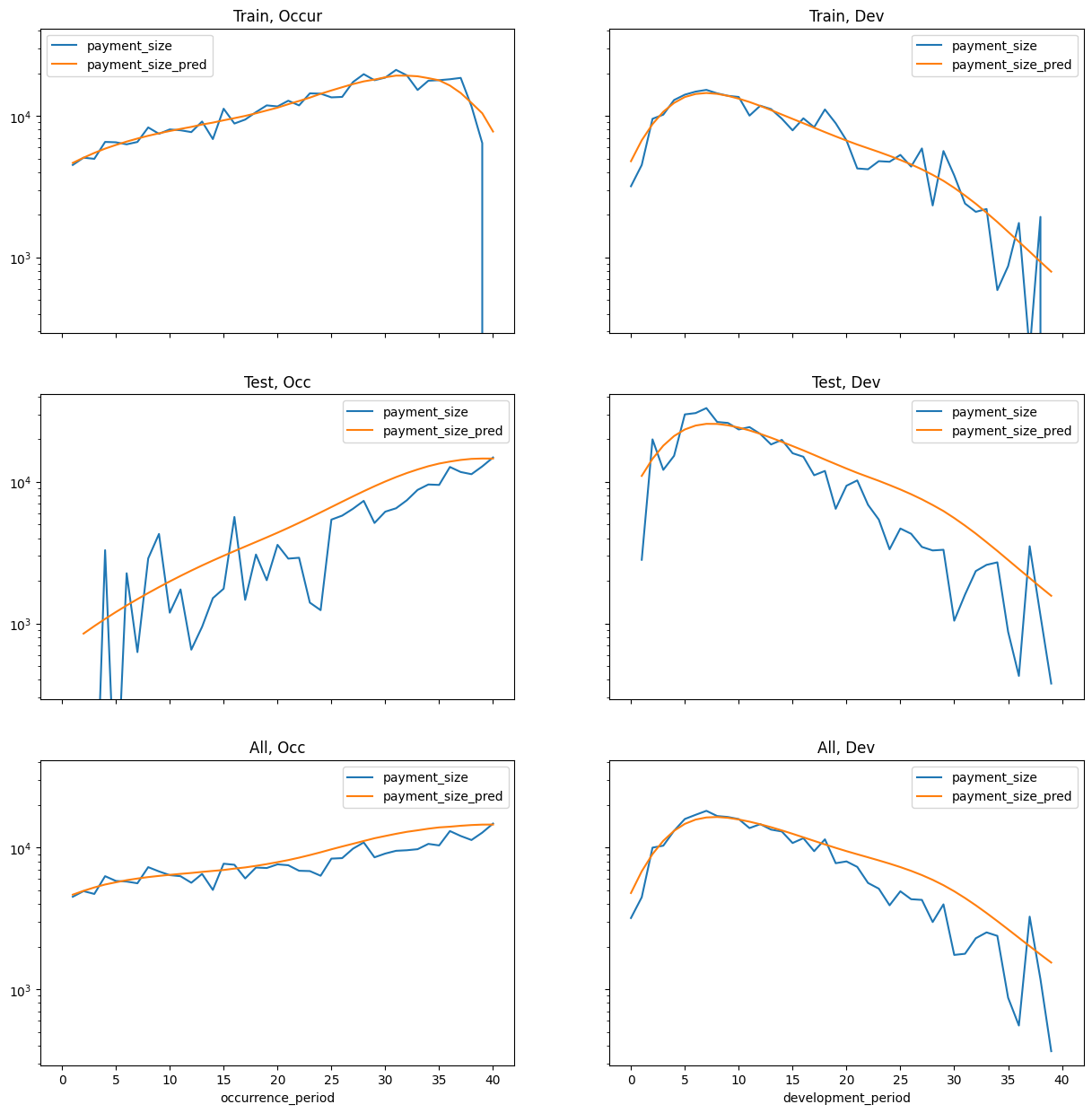

This should look reasonable.

Neural Network, Occurence/Development Only

Can we have deep learning just figure out this curve by using the periods as numeric inputs, rather than the one-hot encoding?

Here we have a ResNet pretty similar to the ones previously used in the other notebooks. There is more functionality built-in than a base ResNet - some observations on the architecture:

• This is the concatenation variant rather than addition variant of the ResNet, but for a single hidden layer it does not make much difference.
• Batch Normalisation: We use a variant of FixUp initialisation so the batch normalisation is not needed for numerical stability. Our experience is that including this leads to a higher degree of overfitting.
• L1 and L2 normalisation are built into the sci-kit learn wrapper. L1 enforces sparsity but also leads to some underfitting of effects.
• Dropout layer is available for optimisation.
• One Cycle learning schedule with Adam is used as the optimiser in the sci-kit learn wrapper above. It seems to work in getting a working model quickly.
• ELU is used as activation. Sigmoid does not appear to work well. Occasionally ReLU has dead neurons which impact model results due to low neuron count.

class LogLinkResNet(nn.Module):
    # Define the parameters in __init__
    def __init__(
        self,      
        n_input,                                           # number of inputs
        n_output,                                          # number of outputs
        init_bias,                                         # init mean value to speed up convergence 
        n_hidden,                                          # hidden layer size
        batch_norm,                                        # whether to do batch norm (boolean)
        dropout,                                           # dropout percentage,
        **kwargs, 
    ): 

        super(LogLinkResNet, self).__init__()

        self.hidden = nn.Linear(n_input, n_hidden)   # Hidden layer

        # Batchnorm layer    
        self.batch_norm = batch_norm
        if batch_norm:
            self.batchn = nn.BatchNorm1d(n_hidden)       
        self.dropout = nn.Dropout(dropout)
        self.linear = torch.nn.Linear(n_input, n_output)   # Linear coefficients

        # Neural net coefficients - no bias - glm has a bias already
        self.neural = torch.nn.Linear(n_hidden, n_output, bias=False)  

        nn.init.zeros_(self.linear.weight)                 # Initialise to zero
        nn.init.zeros_(self.neural.weight)                 # n.b. do not initialise hidden layers to zero
        self.linear.bias.data = torch.tensor(init_bias)


    # The forward function defines how you get y from X.
    def forward(self, x):
        h = F.elu(self.hidden(x))                   # Apply hidden layer
        if self.batch_norm:
            h = self.batchn(h)                       # Apply batchnorm   
        h = self.dropout(h)
        return torch.exp(self.linear(x) + self.neural(h))  # Add GLM to NN

Development Period Only Model

So here we min-max scale the data rather than one-hot encode it. The ResNet to figure out the effect.

First, we test with a model with only one feature - development_period.

model_NN = Pipeline(
    steps=[
        ("keep", ColumnKeeper(["development_period"])),   # Just development period!
        ('zero_to_one', MinMaxScaler()),       # Important! Standardize deep learning inputs.
        ("model", TabularNetRegressor(LogLinkResNet, n_hidden=20, max_iter=nn_iter, max_lr=0.05))
    ]
)

model_NN.fit(
    dat.loc[dat.train_ind == 1],
    dat.loc[dat.train_ind == 1, ["payment_size"]]
)

Train RMSE:  55491.70703125  Train Loss:  -76383.375
Train RMSE:  55438.2109375  Train Loss:  -76925.859375
Train RMSE:  55411.64453125  Train Loss:  -77013.7578125
Train RMSE:  55366.9921875  Train Loss:  -77228.1640625
Train RMSE:  55359.65234375  Train Loss:  -77283.15625
Train RMSE:  55358.203125  Train Loss:  -77291.875
Train RMSE:  55357.453125  Train Loss:  -77296.515625
Train RMSE:  55356.91015625  Train Loss:  -77299.859375
Train RMSE:  55356.59375  Train Loss:  -77301.8515625
Train RMSE:  55356.45703125  Train Loss:  -77302.671875

Pipeline(steps=[('keep', ColumnKeeper(cols=['development_period'])),
                ('zero_to_one', MinMaxScaler()),
                ('model',
                 TabularNetRegressor(max_iter=500, max_lr=0.05,
                                     module=<class '__main__.LogLinkResNet'>))])

In a Jupyter environment, please rerun this cell to show the HTML representation or trust the notebook.
On GitHub, the HTML representation is unable to render, please try loading this page with nbviewer.org.

make_model_subplots(model_NN, dat)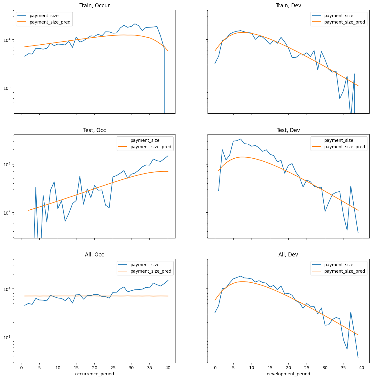

So far, this approach does fine. It seems to reflect the development pattern for the training and holdout datasets. But to replicate chain ladder, we need occurrence too.

Development and Occurrence Model

Now we use both development and occurrence.

model_NN = Pipeline(
    steps=[
        ("keep", ColumnKeeper(["occurrence_period", "development_period"])),   # both
        ('zero_to_one', MinMaxScaler()),       # Important! Standardize deep learning inputs.
        ("model", TabularNetRegressor(LogLinkResNet, n_hidden=20, max_iter=nn_iter, max_lr=0.05))
    ]
)

model_NN.fit(
    dat.loc[dat.train_ind == 1],
    dat.loc[dat.train_ind == 1, ["payment_size"]]
)

Train RMSE:  55491.5390625  Train Loss:  -76383.375
Train RMSE:  55372.53125  Train Loss:  -77204.9765625
Train RMSE:  55350.5703125  Train Loss:  -77285.359375
Train RMSE:  55331.859375  Train Loss:  -77372.9140625
Train RMSE:  55316.28515625  Train Loss:  -77478.140625
Train RMSE:  55297.3515625  Train Loss:  -77553.765625
Train RMSE:  55292.02734375  Train Loss:  -77582.234375
Train RMSE:  55289.3984375  Train Loss:  -77595.484375
Train RMSE:  55288.16796875  Train Loss:  -77602.0078125
Train RMSE:  55287.69140625  Train Loss:  -77604.6171875

Pipeline(steps=[('keep',
                 ColumnKeeper(cols=['occurrence_period',
                                    'development_period'])),
                ('zero_to_one', MinMaxScaler()),
                ('model',
                 TabularNetRegressor(max_iter=500, max_lr=0.05,
                                     module=<class '__main__.LogLinkResNet'>))])

In a Jupyter environment, please rerun this cell to show the HTML representation or trust the notebook.
On GitHub, the HTML representation is unable to render, please try loading this page with nbviewer.org.

dat_nn_pred, triangle_resnet_do = make_pred_set_and_triangle(model_NN, dat.loc[dat.train_ind == 1], dat.loc[dat.train_ind == 0])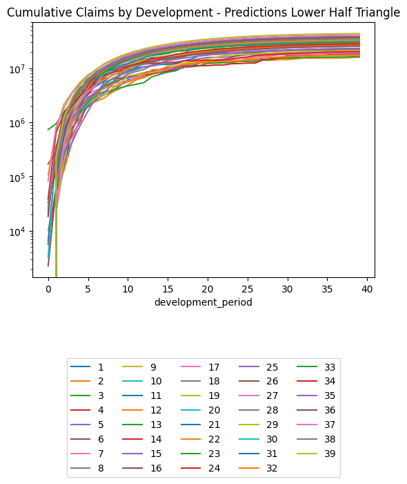

make_model_subplots(model_NN, dat)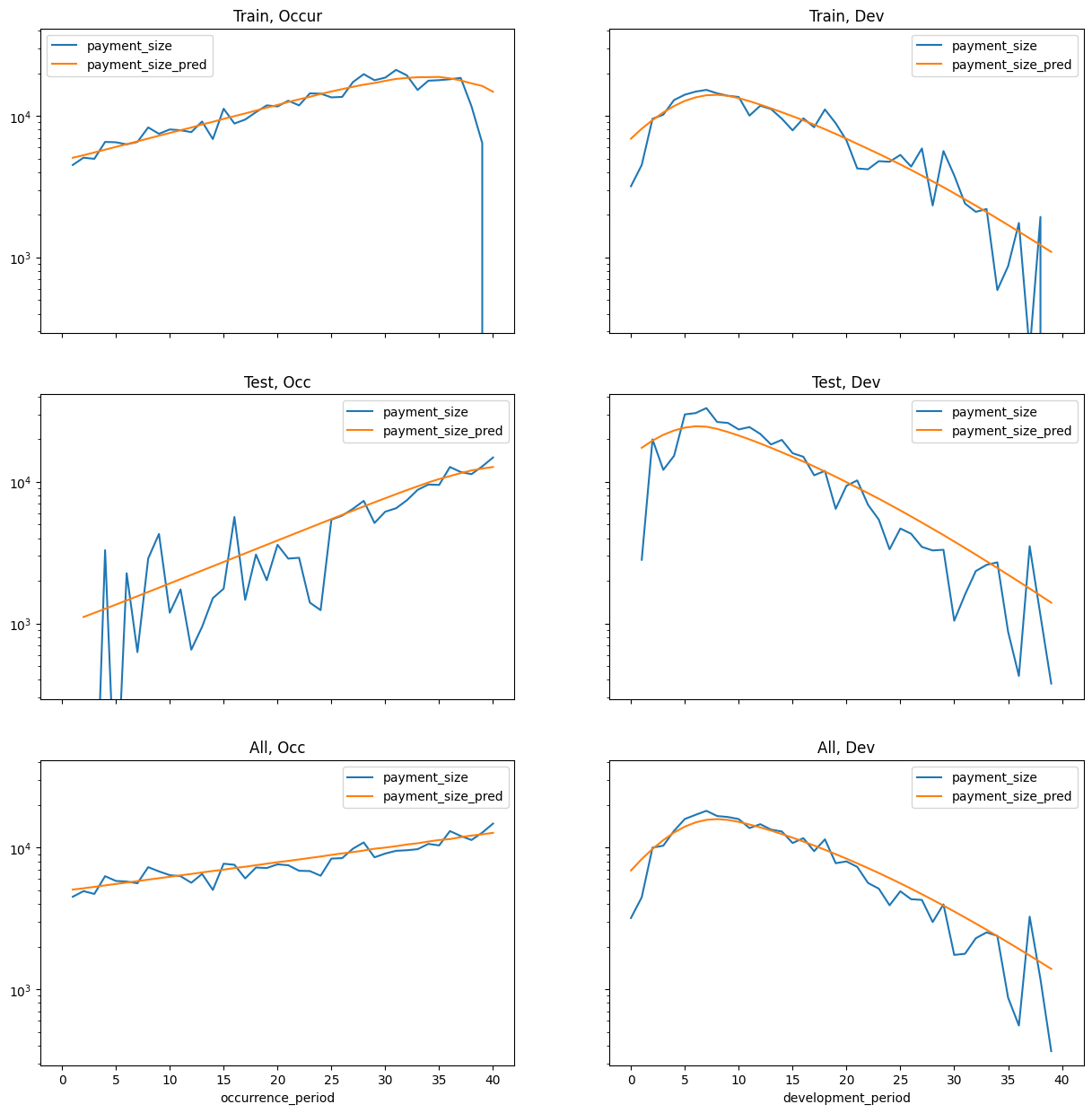

The model does fit well for training data, but the model sometimes appears overfits, particularly on the occurrence period trend for dataset 1, which leads to a deterioration of performance in test data. Performance appears to be better when batch normalisation is not used.

“SplineNet” Architecture, Occurrence/Development Only

An observation with the above model compared to the spline GLM is that all the hidden layer components are naturally interactions rather than the one-way splines in the GLM. If only we could fit the model as a linear combination of one-way effects.

We re-introduce ideas from our earlier paper [1]. This model architecture includes:

• a log-link, through the exponential transformation at the end,
• one-way neural network splines, linearly combined, to ensure single-variable effects are well-captured, similar to the spline-GLM earlier,
• a neural interaction component to which l1, weight decay, dropout regularization and penalties are applied to put a cost to multi-way effects and discourage overfitting.
• an interaction parameter, which can be set at between 0.0 and 1.0, to governs the impact of this interaction. This is set as a trainable parameter with a sigmoid gate based on Residual Gates and Highway Networks [3] so that the model can identify to what extent interactions are required.

class SplineNet(nn.Module):
    # Define the parameters in __init__
    def __init__(
        self,      
        n_input,                                           # number of inputs
        n_output,                                          # number of outputs
        init_bias,                                         # init mean value to speed up convergence 
        n_hidden,                                          # hidden layer size
        dropout,                                           # dropout percentage 
        interactions=0.0,                                  # 0.0 - 1.0 initial weight to apply interactions
        interactions_trainable=True,                       # Whether the model can adapt the interactions weight over time.
        inverse_of_link_fn=torch.exp,
        **kwargs
    ): 
        # Initialise
        super(SplineNet, self).__init__()
        self.interactions=nn.Parameter(
            torch.logit(torch.tensor(interactions), eps=1e-5), 
            requires_grad=interactions_trainable)

        self.n_input = n_input
        self.inverse_of_link_fn = inverse_of_link_fn

        # One-way layers
        self.oneways = nn.ModuleList([nn.Linear(1, n_hidden) for i in range(0, n_input)])
        self.oneway_linear = nn.Linear(n_hidden * n_input, n_output)
        self.oneway_linear.bias.data = torch.tensor(init_bias)    # Initialise bias to speed up convergence
        nn.init.zeros_(self.oneway_linear.weight)                 # n.b. do not initialise hidden layers to zero

        # Optional Interactions Layer
        self.hidden = nn.Linear(n_input, n_hidden)              # Hidden layer - interactions
        self.linear = nn.Linear(n_hidden, n_output, bias=False) # Neural net coefficients
        nn.init.zeros_(self.linear.weight)                 # n.b. do not initialise hidden layers to zero
        
        # Dropout
        self.dropout = nn.Dropout(dropout)   

    # The forward function defines how you get y from X.
    def forward(self, x):
        # Apply one-ways
        chunks = torch.split(x, [1 for i in range(0, self.n_input)], dim=1) 
        splines = torch.cat([self.oneways[i](chunks[i]) for i in range(0, self.n_input)], dim=1)

        # Sigmoid gate
        interact_gate = torch.sigmoid(self.interactions)

        splines_out = self.oneway_linear(F.elu(splines)) * (1 - interact_gate)
        interact_out = self.linear(F.elu(self.hidden(self.dropout(x)))) * (interact_gate)
        
        # Add ResNet style
        return self.inverse_of_link_fn(splines_out + interact_out) 

model_spline_net = Pipeline(
    steps=[
        ("keep", ColumnKeeper(["occurrence_period", "development_period"])),   # both
        ('zero_to_one', MinMaxScaler()),       # Important! Standardize deep learning inputs.
        ("model", TabularNetRegressor(SplineNet, n_hidden=20, max_iter=nn_iter, max_lr=0.05))
    ]
)

model_spline_net.fit(
    dat.loc[dat.train_ind == 1],
    dat.loc[dat.train_ind == 1, ["payment_size"]]
)

Train RMSE:  55489.55078125  Train Loss:  -76383.359375
Train RMSE:  55360.18359375  Train Loss:  -77245.1328125
Train RMSE:  55355.15234375  Train Loss:  -77276.9140625
Train RMSE:  55335.62109375  Train Loss:  -77348.296875
Train RMSE:  55298.7421875  Train Loss:  -77537.8125
Train RMSE:  55291.6015625  Train Loss:  -77573.96875
Train RMSE:  55289.71875  Train Loss:  -77584.609375
Train RMSE:  55281.45703125  Train Loss:  -77640.9296875
Train RMSE:  55279.375  Train Loss:  -77654.7109375
Train RMSE:  55278.79296875  Train Loss:  -77659.125

Pipeline(steps=[('keep',
                 ColumnKeeper(cols=['occurrence_period',
                                    'development_period'])),
                ('zero_to_one', MinMaxScaler()),
                ('model',
                 TabularNetRegressor(max_iter=500, max_lr=0.05,
                                     module=<class '__main__.SplineNet'>))])

In a Jupyter environment, please rerun this cell to show the HTML representation or trust the notebook.
On GitHub, the HTML representation is unable to render, please try loading this page with nbviewer.org.

dat_nn_pred, triangle_nn_spline = make_pred_set_and_triangle(model_spline_net, dat.loc[dat.train_ind == 1], dat.loc[dat.train_ind == 0])

make_model_subplots(model_spline_net, dat)

Mixture Density Network

In Probabilistic Forecasting with Neural Networks Applied to Loss Reserving [2], Muhammed Al-Mudafer introduced the idea of a “ResMDN” model which produces results similar to a more advanced stochastic chain ladder that has a deep learning component. The ResMDN extends the one-hot GLM into a ResNet, then predicts a full probability distribution using Mixture Density Networks.

We note that our “SplineNet” architecture appears to compare well to the one-hot GLM, since it fits curves to the features rather than one-hot encoding each occurrence and development period. So we will add MDN output and loss build on the “SplineNet” model instead of the GLM.

Distribution Assumption

The Mixture Density Network models the output as being a mixture of normal distributions. However, it becomes quickly apparent the normal distribution is not a good fit for individual claims data. The SPLICE claim payments, like typical insurance claims data, is heavily skewed:

plt.hist((dat.loc[(dat.train_ind == 1) & (dat.payment_size > 0), ["payment_size"]]))

(array([1.2441e+04, 2.5600e+02, 4.8000e+01, 2.5000e+01, 7.0000e+00,
        4.0000e+00, 3.0000e+00, 0.0000e+00, 1.0000e+00, 1.0000e+00]),
 array([5.43023949e+01, 3.13449125e+05, 6.26843938e+05, 9.40238750e+05,
        1.25363362e+06, 1.56702838e+06, 1.88042325e+06, 2.19381800e+06,
        2.50721275e+06, 2.82060775e+06, 3.13400250e+06]),
 <BarContainer object of 10 artists>)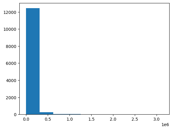

Given the skew, plot log-transformed histogram:

plt.hist(np.log(dat.loc[(dat.train_ind == 1) & (dat.payment_size > 0), ["payment_size"]]))

(array([  13.,   27.,   58., 1162., 4850., 4191.,  902., 1315.,  233.,
          35.]),
 array([ 3.99456835,  5.09089375,  6.18721914,  7.28354454,  8.37986946,
         9.47619534, 10.57252026, 11.66884613, 12.76517105, 13.86149693,
        14.95782185]),
 <BarContainer object of 10 artists>)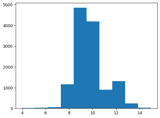

It is clear from the plot that the log-normal distribution should be more appropriate than the normal for the distribution of payments in individual claims data.

Consequently, we propose an adjusted log-normal MDN approach, which also takes into account the observations with zero payments: 1. Calculate point estimates as \(exp(\mu + \sigma^2/2)\), being mean of a log-normal, 2. Apply loss to \(log(y + \epsilon)\) rather than \(y\) (with \(\epsilon\) being some small value), 3. Use \(\sqrt ReLU\) + \(\epsilon\) as the activation for \(\sigma\) rather than \(exp\).

This design, which appears to be novel, addresses two numerical stability challenges from having observations with zero payment: * Mean of the zero records is zero. This means typically, with a log-link \(log(0), \rightarrow -\infty\). Adding the \(\epsilon\) value avoids this. * \(\sigma\) of the zero records is also zero. Typically, MDNs use an exponential or ELU activation for \(sigma\), so again \(log(0) \rightarrow -\infty\). Use of ReLU allows \(sigma\) to be extremely small without numerical instability. * Apply square root \(\sigma\) to avoid any unintended quadratic effects to \(exp(\mu + \sigma^2/2)\)

Loss function

Our adjusted Mixture Density Networks loss function is as follows. This utilises the torch.logsumexp function for the best numerical stability.

SMALL = 1e-7

def log_mdn_loss_fn(y_dists, y):
    y = torch.log(y + SMALL)        # log(y) ~ Normal
    alpha, mu, sigma = y_dists
    m = torch.distributions.Normal(loc=mu, scale=sigma) # Normal
    loss = -torch.logsumexp(m.log_prob(y) + torch.log(alpha + 1e-15), dim=-1)
    return torch.mean(loss) # Average over dataset

Meanwhile it is possible to get similar result as the point estimate MDN model using this loss function, which calculates the Poisson NLL loss:

def point_poisson_nll_loss(y_dists, y):
    alpha, mu, sigma = y_dists
    yhat = torch.sum(alpha * torch.exp(mu + 0.5 * sigma * sigma), dim=1).unsqueeze(1)
    assert yhat.size() == y.size()
    return F.poisson_nll_loss(yhat, y, log_input=False, full=False, eps=1e-8, reduction='mean')

It is possible to train for both losses by summing both losses as per below. This seems to provide a more reliably stable result for the point estimates than relying on solely the MDN loss, however we found the variational predictions became less accurate so we abandoned this approach.

two_loss = lambda y_dists, y: log_mdn_loss_fn(y_dists, y) + point_poisson_nll_loss(y_dists, y)

Architecture

We take the “SplineNet” architecture presented earlier and use one to provide the point estimates, exactly as before, then apply a second SplineNet module to predict the distributional assumptions. The \(\alpha\), \(\mu\), and \(\sigma\) outputs are calculated in a way such that: * \(\mu\) is calculated with scaling factors to ensure the mean, being \(\Sigma^n_1 (\alpha \times exp(\mu + 0.5 \sigma^2))\), is always equal to the point estimate output, * \(\sigma\) is calculated using ReLU and square root transformation as described above.

We found that whilst optimising for the MDN loss function was often effective, there were training runs when the MSE and point estimates would behave oddly during the training process. Since the estimate for the mean comes directly from a SplineNet sub-module, it is possible to use the previously trained model and weights. This would avoid another source of instability. An interesting observation with this is that a similar approach could be used to add distributional predictions to any point estimate model.

class LognormalSplineMDN(nn.Module):  # V3
    # Define the parameters in __init__
    def __init__(
        self,      
        n_input,                                           # number of inputs
        n_output,                                          # number of outputs
        init_bias,                                         # init mean value to speed up convergence
        init_extra,                                        # init mean value to speed up convergence
        n_hidden,                                          # hidden layer size
        dropout,                                           # dropout percentage 
        n_gaussians,                                       # number of gaussians
        interactions=0.0,                                      # 0.0 - 1.0 whether to apply interactions
        point_estimates=False,
        **kwargs
    ): 
        assert n_output==1, "Not implemented for n_output > 1"

        # Initialise
        super(LognormalSplineMDN, self).__init__()
        self.n_gaussians = n_gaussians
        self.point_estimates = point_estimates
        self.point_estimator = SplineNet(
            n_output=1, init_bias=init_bias, inverse_of_link_fn=lambda x: x,
            # the other parameters are passed straight through:
            n_input=n_input, n_hidden=n_hidden, dropout=dropout, interactions=interactions, 
        )
        self.point_estimator.load_state_dict(init_extra[0])
        self.point_estimator.requires_grad_(False)

        self.distribution_estimator = SplineNet(
            n_output=3 * n_gaussians, init_bias=init_extra[1], inverse_of_link_fn=lambda x: x,
            # the other parameters are passed straight through:
            n_input=n_input, n_hidden=n_hidden, dropout=dropout, interactions=interactions, 
        )        

    # The forward function defines how you get y from X.
    def forward(self, x):
        predictor = self.point_estimator(x)

        if self.point_estimates:        
            return torch.exp(predictor)
        else:
                alpha0, median0, sigma0 = torch.split(
                    self.distribution_estimator(x), 
                    [self.n_gaussians, self.n_gaussians, self.n_gaussians], 
                    dim=1
                )

                # Alpha: Softmax so it sums to 100%
                alpha = F.softmax(alpha0, dim=-1)
                log_mix_prob = torch.log(alpha + 1e-15)

                # Sigma: ReLU with minimum of SMALL
                s2 = F.relu(sigma0) + SMALL
                sigma = torch.sqrt(s2)

                # Linear predictors. sum of alpha * exp(mdn_lin_preds) = exp(lin_pred)
                # Adjust to make sure they equate.
                log_scaling_factor = torch.logsumexp(log_mix_prob + median0, dim=-1).unsqueeze(1) - predictor

                # Mean is exp(mu + 0.5 * sigma^2)
                mu = median0 - log_scaling_factor - 0.5 * s2                                               

                return alpha, mu, sigma
                

Number of distributions

We will make a generic assumption for three distributions being: 1. Zeroes (most records are zero payment at this granular claim/period level), 2. Minor payments, and 3. Major payments

More distributions can be used e.g. when there are several peril categories, but assuming the presence of these three seems generally reasonable.

Initialisation

We will need to initialise our model intelligently for numerical stability and faster convergence.

For the initial values, we will assume large claims are 5% of the claims and 10x larger than the average, the model will train this to the right levels.

percent_zeroes = (dat.loc[(dat.train_ind == 1) & (dat.payment_size < 0.001)].claim_no.count()) / (dat.loc[(dat.train_ind == 1)].claim_no.count())
mean_log_payment = np.log(dat.loc[(dat.train_ind == 1) & (dat.payment_size > 0), ["payment_size"]].values).mean()

mean_payment_encl_zeroes = dat.loc[(dat.train_ind == 1) & (dat.payment_size > 0), ["payment_size"]].values.mean()
mean_payment_incl_zeroes = dat.loc[(dat.train_ind == 1), ["payment_size"]].values.mean()

sigma_payment = np.sqrt((np.log(mean_payment_encl_zeroes) - mean_log_payment) * 2)

mdn_init_bias = np.array([
    # Alpha
    np.log(percent_zeroes),
    np.log((1-percent_zeroes) * 0.95),
    np.log((1-percent_zeroes) * 0.05),
    # Mu
    np.log(SMALL),
    mean_log_payment + np.log(0.526),
    mean_log_payment + np.log(10),
    # Sigma
    -1.0,
    sigma_payment,
    sigma_payment,
], dtype=np.float32)

{
    "Percent of records zeroes": percent_zeroes, 
    "Alpha bias after softmax": F.softmax(torch.tensor(mdn_init_bias[0:3]),dim=-1),  # This should return the correct zero percentage
    "Mean log payment": mean_log_payment, 
    "Sigma (non-zero claims)": sigma_payment,
    "Mean payment (excl zeroes)": mean_payment_encl_zeroes,
    "Mean Payment (incl zeroes)": mean_payment_incl_zeroes
}

{'Percent of records zeroes': 0.8141110448802756,
 'Alpha bias after softmax': tensor([0.8141, 0.1766, 0.0093]),
 'Mean log payment': 9.755892,
 'Sigma (non-zero claims)': 1.4647239534347847,
 'Mean payment (excl zeroes)': 50443.03,
 'Mean Payment (incl zeroes)': 9376.803}

Model fitting

Fit the MDN below, with some validation checks that the module and initialisation has been performed correctly.

model_spline_mdn = Pipeline(
    steps=[
        ("keep", ColumnKeeper(["occurrence_period", "development_period"])),   # both
        ('zero_to_one', MinMaxScaler()),       # Important! Standardize deep learning inputs.
        ("model", TabularNetRegressor(
                LognormalSplineMDN, 
                n_hidden=20, 
                max_iter=mdn_iter, 
                max_lr=0.025, 
                n_gaussians=3,
                criterion=log_mdn_loss_fn,
                init_extra=[model_spline_net["model"].module_.state_dict(), mdn_init_bias],
                # clip_value=3.0,
                keep_best_model=True  # Noting numerical stability, keep the best model instead
            )
        )
    ]
)

# Fit model
model_spline_mdn.fit(
    dat.loc[dat.train_ind == 1],
    dat.loc[dat.train_ind == 1, ["payment_size"]]
)

Train RMSE:  55278.71875  Train Loss:  181.297119140625
Train RMSE:  55278.71875  Train Loss:  47.793006896972656
Train RMSE:  55278.71875  Train Loss:  4.475003242492676
Train RMSE:  55278.71875  Train Loss:  2.6302762031555176
Train RMSE:  55278.71875  Train Loss:  2.598949432373047
Train RMSE:  55278.71875  Train Loss:  2.5837700366973877
Train RMSE:  55278.71875  Train Loss:  2.5708096027374268
Train RMSE:  55278.71875  Train Loss:  2.5611422061920166
Train RMSE:  55278.71875  Train Loss:  2.555274724960327
Train RMSE:  55278.71875  Train Loss:  2.5528206825256348

Pipeline(steps=[('keep',
                 ColumnKeeper(cols=['occurrence_period',
                                    'development_period'])),
                ('zero_to_one', MinMaxScaler()),
                ('model',
                 TabularNetRegressor(criterion=<function log_mdn_loss_fn at 0x2bc8eeb00>,
                                     init_extra=[OrderedDict([('interactions',
                                                               tensor(-5.0061)),
                                                              ('oneways.0.weight',
                                                               tensor([[-0.0981],
        [-0.6153],
        [-0.0221],
        [-0.5114],
        [ 0.0978],
        [ 0.6668],
        [ 0.1500],
        [...
                                                               tensor([[ 3.2120, -6.1099, -6.2423, -6.5094, -3.1338,  7.8484,  2.6359,  6.3528,
          4.7452, -5.0441,  7.7757, -3.3306,  3.7796,  4.8792,  6.3781, -4.6370,
         -0.9826, -4.2656, -6.8903, -4.4056]]))]),
                                                 array([ -0.20565851,  -1.7338991 ,  -4.678338  , -16.118095  ,
         9.113438  ,  12.058476  ,  -1.        ,   1.464724  ,
         1.464724  ], dtype=float32)],
                                     keep_best_model=True, max_iter=500,
                                     max_lr=0.025,
                                     module=<class '__main__.LognormalSplineMDN'>))])

In a Jupyter environment, please rerun this cell to show the HTML representation or trust the notebook.
On GitHub, the HTML representation is unable to render, please try loading this page with nbviewer.org.

Check point estimates:

# Lower half triangle predictions
dat_mdn_pred, triangle_mdn_spline = make_pred_set_and_triangle(model_spline_mdn, dat.loc[dat.train_ind == 1], dat.loc[dat.train_ind == 0])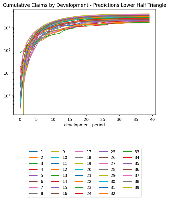

make_model_subplots(model_spline_mdn, dat)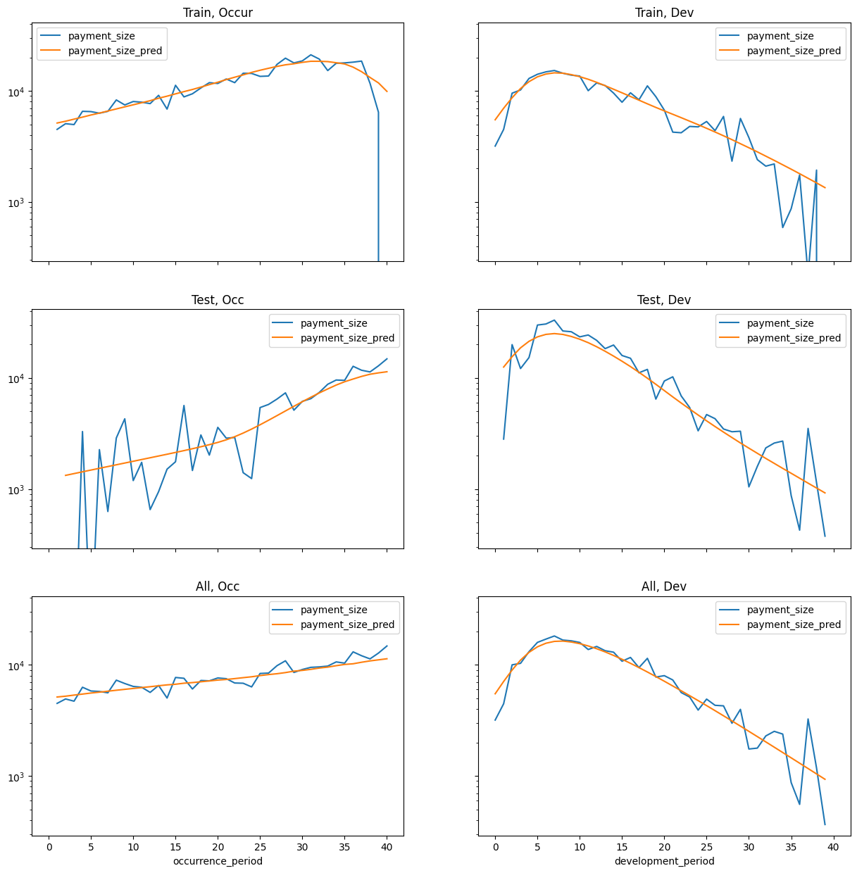

Check probabilistic predictions

def make_distribution_subplots(model):
    fig, axes = plt.subplots(2, 3, sharex='col', sharey=False, figsize=(15, 7))

    axes[0,0].title.set_text("All claims")
    axes[0,1].title.set_text("Non-zero claims")
    axes[0,2].title.set_text("Log non-zero claims")

    axes[0,0].hist((dat.loc[(dat.train_ind == 1), ["payment_size"]]))
    axes[0,1].hist((dat.loc[(dat.train_ind == 1) & (dat.payment_size > 0), ["payment_size"]]))
    axes[0,2].hist(np.log(dat.loc[(dat.train_ind == 1) & (dat.payment_size > 0), ["payment_size"]]))

    alpha, mu, sigma = model.predict(dat.loc[(dat.train_ind == 1)], point_estimates=False)

    categorical = torch.distributions.Categorical(alpha)
    alpha_sample = categorical.sample().unsqueeze(1)
    n_01 = Variable(sigma.data.new(sigma.size(0), 1).normal_())
    sample = mu.gather(1, alpha_sample) + n_01 * sigma.gather(1, alpha_sample) 
    sample = np.exp(sample.cpu().detach().numpy())

    axes[1,0].hist(sample)
    axes[1,1].hist(sample[sample > 0.01])
    axes[1,2].hist(np.log(sample[sample > 0.01]))

make_distribution_subplots(model_spline_mdn)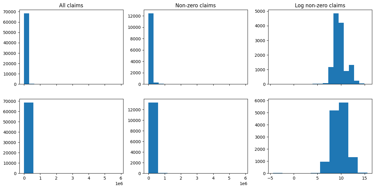

We should hopefully see a resemblance between the distributions.

Cross Validation and Hyperparameter Search

Rolling Origin Validation

The problem with using a random split for cross validation is that records may pertain to the same time period, but we are predicting records that are completely out of the time period.

It’s fairly simple to implement a payment period based cross validation using PredefinedSplit:

ps = PredefinedSplit(nn_train.cv_ind)

However, this did not lead to good quality results in our testing, so we will implement the rolling origin validation.

class RollingOriginSplit:
    def __init__(self, start_cut, n_splits):
        self.start_cut = start_cut
        self.n_splits = n_splits

    def split(self, X=None, y=None, groups=None):
        """Generate indices to split data into training and test set.
        Parameters
        ----------
        X : array-like of shape (n_samples, n_features)
            Training data, where `n_samples` is the number of samples
            and `n_features` is the number of features.
        y : array-like of shape (n_samples,)
            Always ignored, exists for compatibility.
        groups : array-like of shape (n_samples,)
            Payment period for splits
        Yields
        ------
        train : ndarray
            The training set indices for that split.
        test : ndarray
            The testing set indices for that split.
        """
        quantiles = pd.qcut(groups, self.start_cut + self.n_splits + 1, labels=False)

        for split_value in range(self.start_cut, self.start_cut + self.n_splits):
            yield np.where(quantiles <= split_value)[0], np.where(quantiles == split_value + 1)[0]

ps = RollingOriginSplit(5, 5).split(groups=dat.loc[dat.train_ind == 1].payment_period)
for tr, te in ps:
    print(len(tr), len(te), len(tr)+ len(te) )

37921 8376 46297
46297 6001 52298
52298 6336 58634
58634 6687 65321
65321 3462 68783

len(dat.loc[dat.train_ind == 1].index)

68783

Random Search:

Use Random Search - noting comments here about the limited benefits of Bayesian Search.

• l1 penalty, weight decay: Cap at 0.1 to avoid underfitting problems.
• dropout: try higher percentages.
• number of neurons in hidden layer: keep relatively small, the data is not that complex
• interactions: test with and without.
• max iter, max lr: - keep at these values or similar to get something close to convergence in a short number of iterations

parameters_nn = {
    "l1_penalty": [0.0, 0.001, 0.01, 0.1],
    "weight_decay": [0.0, 0.001, 0.01, 0.1],
    "n_hidden": [5, 10, 20],
    # "interactions": [0.0, 0.25, 0.5, 0.75, 1.0],
    "dropout": [0, 0.25, 0.5],
    "max_iter": [nn_cv_iter],
    "max_lr": [0.05],
    "verbose": [0],
    "clip_value": [None, 3.0],
    "keep_best_model": [True] 
}

model_NN_CV = Pipeline(
    steps=[
        ("keep", ColumnKeeper(["occurrence_period", "development_period"])),  
        ('zero_to_one', MinMaxScaler()),       # Important! Standardize deep learning inputs.
        ("model", RandomizedSearchCV(
            TabularNetRegressor(SplineNet),
            parameters_nn,
            n_jobs=4,  # Run in parallel (small model)
            n_iter=cv_runs, # Models train slowly, so try only a few models
            cv=RollingOriginSplit(5,5).split(groups=dat.payment_period.loc[dat.train_ind == 1]),
            random_state=42,
            refit=False
        )),
    ]
)

model_NN_CV.fit(
    dat.loc[dat.train_ind == 1],
    dat.loc[dat.train_ind == 1, ["payment_size"]]
)


bst_nn = model_NN_CV["model"].best_params_
print("best parameters:", bst_nn)

cv_results = pd.DataFrame(model_NN_CV["model"].cv_results_)

# Refit best model for longer iters
model_NN_CV = Pipeline(
    steps=[
        ("keep", ColumnKeeper(["occurrence_period", "development_period"])),  
        ('zero_to_one', MinMaxScaler()),       # Important! Standardize deep learning inputs.
        ("model", TabularNetRegressor(
                SplineNet, 
                l1_penalty=bst_nn["l1_penalty"],
                weight_decay=bst_nn["weight_decay"],  
                n_hidden=bst_nn["n_hidden"],   
                # interactions=bst_nn["interactions"],
                dropout=bst_nn["dropout"],                             
                max_iter=nn_iter, 
                max_lr=bst_nn["max_lr"], 
            )
        )
    ]
)
model_NN_CV.fit(
    dat.loc[dat.train_ind == 1],
    dat.loc[dat.train_ind == 1, ["payment_size"]]
)

best parameters: {'weight_decay': 0.01, 'verbose': 0, 'n_hidden': 10, 'max_lr': 0.05, 'max_iter': 100, 'l1_penalty': 0.0, 'keep_best_model': True, 'dropout': 0.5, 'clip_value': None}
Train RMSE:  55491.87890625  Train Loss:  -76383.359375
Train RMSE:  55388.3046875  Train Loss:  -77174.5
Train RMSE:  55351.515625  Train Loss:  -77285.703125
Train RMSE:  55333.53515625  Train Loss:  -77376.625
Train RMSE:  55301.0390625  Train Loss:  -77523.671875
Train RMSE:  55292.10546875  Train Loss:  -77570.9921875
Train RMSE:  55290.66796875  Train Loss:  -77579.3359375
Train RMSE:  55289.921875  Train Loss:  -77583.3203125
Train RMSE:  55289.45703125  Train Loss:  -77585.7421875
Train RMSE:  55289.2578125  Train Loss:  -77586.828125

Pipeline(steps=[('keep',
                 ColumnKeeper(cols=['occurrence_period',
                                    'development_period'])),
                ('zero_to_one', MinMaxScaler()),
                ('model',
                 TabularNetRegressor(dropout=0.5, max_iter=500, max_lr=0.05,
                                     module=<class '__main__.SplineNet'>,
                                     n_hidden=10, weight_decay=0.01))])

In a Jupyter environment, please rerun this cell to show the HTML representation or trust the notebook.
On GitHub, the HTML representation is unable to render, please try loading this page with nbviewer.org.

make_model_subplots(model_NN_CV, dat)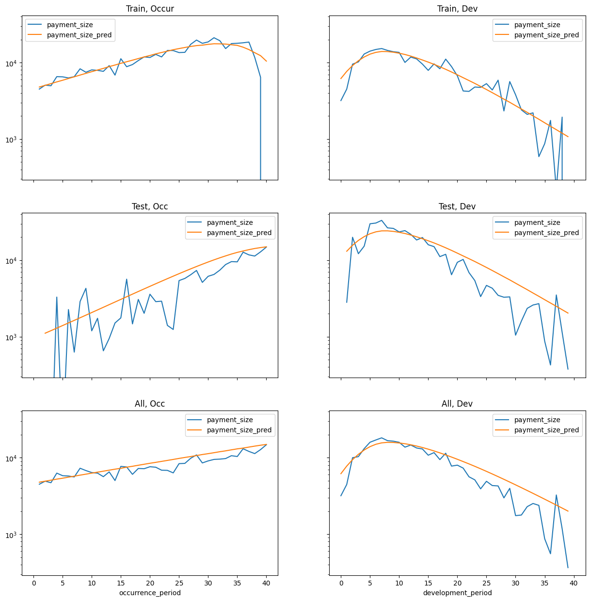

More predictions and diagnostics

dat_nn_pred, triangle_nn_cv = make_pred_set_and_triangle(model_NN_CV, dat.loc[dat.train_ind == 1], dat.loc[dat.train_ind == 0])

(triangle_nn_cv
    .loc[lambda df: df.occurrence_period != cutoff]
    .pivot(index = "development_period", columns = "occurrence_period", values = "payment_size_cumulative")
    .plot(logy=True)
)
plt.legend(loc="lower center", bbox_to_anchor=(0.5, -0.8), ncol=5)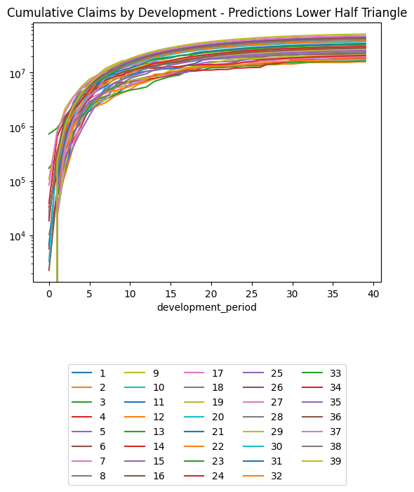

<matplotlib.legend.Legend at 0x2bc947b80>

(dat_nn_pred.loc[lambda df: ~df.train_ind]
    .groupby(["occurrence_period", "development_period", "payment_period"], as_index=False)
    .agg({"payment_size_cumulative": "sum", "payment_size": "sum"})
    .sort_values(by=["occurrence_period", "development_period"])
    .loc[lambda df: df.occurrence_period != cutoff]
    .pivot(index = "development_period", columns = "occurrence_period", values = "payment_size_cumulative")
    .plot(logy=True)
)
plt.legend(loc="lower center", bbox_to_anchor=(0.5, -0.8), ncol=5)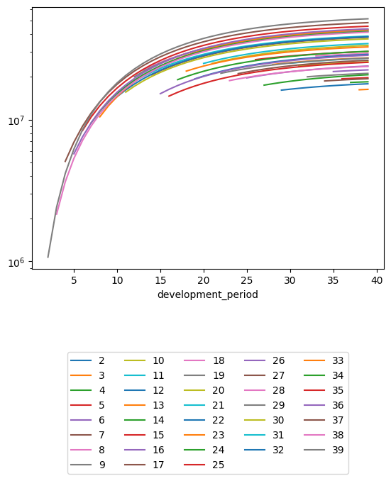

<matplotlib.legend.Legend at 0x2b2b26920>

(dat_nn_pred.loc[lambda df: ~df.train_ind]
    .groupby(["occurrence_period", "development_period", "payment_period"], as_index=False)
    .agg({"payment_size_cumulative": "sum", "payment_size": "sum"})
    .sort_values(by=["occurrence_period", "development_period"])
    .loc[lambda df: df.occurrence_period != cutoff]
    .pivot(index = "development_period", columns = "occurrence_period", values = "payment_size")
    .plot(logy=True)
)
plt.legend(loc="lower center", bbox_to_anchor=(0.5, -0.8), ncol=5)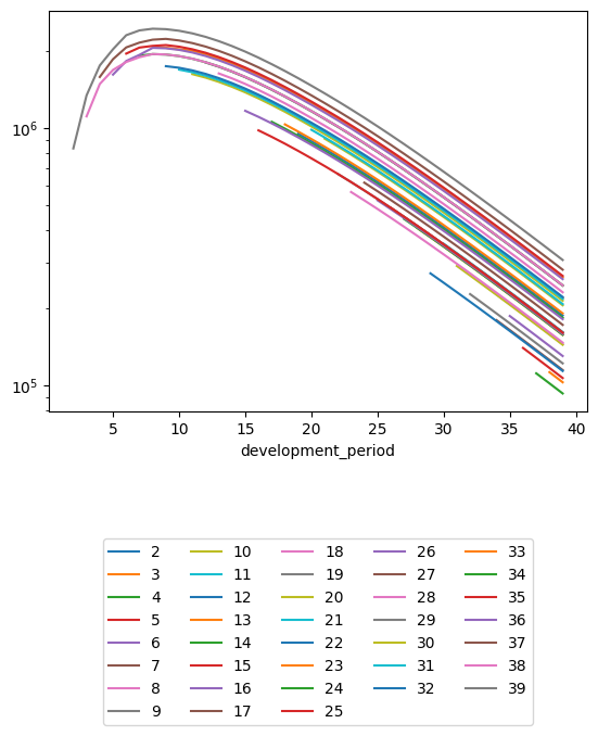

<matplotlib.legend.Legend at 0x2b3e85060>

(triangle_nn_cv.pivot(index = "occurrence_period", columns = "development_period", values = "payment_size_cumulative") - 
triangle_cl.pivot(index = "occurrence_period", columns = "development_period", values = "payment_size_cumulative"))

development_period	0	1	2	3	4	5	6	7	8	9	...	30	31	32	33	34	35	36	37	38	39
occurrence_period
1	0.00	0.00	0.02	0.00	0.00	0.00	0.00	0.25	0.00	0.00	...	0.00	0.00	0.00	0.00	0.00	0.00	0.00	0.00	0.00	0.00
2	0.00	0.00	0.00	0.03	0.00	0.12	0.00	0.00	0.00	0.00	...	0.00	0.00	0.00	0.00	0.00	0.00	0.00	1.00	0.00	93,131.00
3	0.00	0.00	0.00	0.00	0.00	0.00	0.00	0.00	0.00	0.00	...	0.00	0.00	0.00	0.00	0.00	0.00	0.00	0.00	-64,598.00	38,252.00
4	0.00	-0.00	0.00	0.00	0.00	0.00	0.00	0.00	0.00	0.00	...	0.00	0.00	0.00	0.00	0.00	0.00	0.00	88,980.00	-9,110.00	83,940.00
5	0.00	0.00	0.00	0.00	0.00	0.12	0.00	0.00	0.00	0.00	...	0.00	0.00	2.00	0.00	0.00	0.00	-40,644.00	63,272.00	-33,622.00	73,202.00
6	0.00	0.00	0.00	0.00	0.00	0.00	0.00	0.00	0.00	0.00	...	0.00	0.00	0.00	0.00	0.00	88,402.00	55,026.00	183,736.00	84,830.00	214,934.00
7	0.00	0.00	0.00	0.00	0.00	0.00	0.00	-0.25	-0.50	0.00	...	0.00	0.00	0.00	0.00	123,190.00	203,302.00	178,360.00	292,464.00	210,556.00	325,294.00
8	0.00	0.00	0.00	0.00	0.00	0.00	0.00	0.00	0.00	0.00	...	0.00	0.00	0.00	-68,508.00	72,516.00	151,964.00	75,346.00	213,344.00	56,508.00	201,310.00
9	0.00	0.00	0.00	0.00	0.00	0.00	0.00	0.00	0.00	0.00	...	0.00	0.00	19,458.00	530.00	129,638.00	212,160.00	180,378.00	300,830.00	207,586.00	329,414.00
10	0.00	0.00	0.00	0.00	0.00	0.00	0.25	0.00	0.00	0.00	...	0.00	8,376.00	25,792.00	-2,652.00	148,164.00	243,146.00	200,474.00	342,026.00	225,828.00	369,690.00
11	0.00	0.00	0.06	0.00	0.00	0.00	0.00	0.50	0.00	0.00	...	-110,566.00	-84,060.00	-49,410.00	-64,744.00	108,826.00	222,028.00	188,162.00	348,732.00	235,008.00	396,310.00
12	0.00	0.00	0.00	0.00	-0.12	0.00	0.00	0.00	0.00	0.00	...	-239,897.00	-208,423.00	-172,688.00	-171,140.00	-45,364.00	39,498.00	26,048.00	140,704.00	72,844.00	186,628.00
13	0.00	0.00	0.00	0.00	0.00	0.00	0.00	0.00	0.00	0.00	...	-324,870.00	-311,592.00	-288,906.00	-316,024.00	-150,024.00	-44,542.00	-87,842.00	67,404.00	-55,680.00	101,642.00
14	0.00	0.00	0.00	-0.12	0.25	0.00	0.00	0.00	0.00	0.00	...	-8,586.00	86,876.00	182,180.00	234,580.00	422,040.00	559,716.00	583,550.00	747,702.00	704,150.00	861,450.00
15	0.00	0.00	0.00	0.00	0.00	0.00	0.00	0.00	0.00	0.00	...	-982,604.00	-1,005,588.00	-1,014,728.00	-1,077,710.00	-918,006.00	-824,770.00	-898,744.00	-744,430.00	-905,256.00	-744,854.00
16	0.00	0.00	0.00	0.25	0.00	0.00	0.00	0.00	0.00	0.00	...	-282,120.00	-224,990.00	-163,476.00	-148,460.00	30,198.00	153,602.00	145,724.00	306,866.00	225,208.00	383,688.00
17	0.00	0.00	0.00	0.00	0.00	0.00	0.00	0.00	0.00	0.00	...	-256,492.00	-197,700.00	-133,780.00	-120,570.00	72,406.00	205,028.00	193,880.00	368,340.00	276,680.00	448,600.00
18	0.00	0.00	0.00	0.00	0.00	0.00	0.00	0.00	0.00	0.00	...	-370,818.00	-338,750.00	-300,200.00	-306,432.00	-146,528.00	-40,474.00	-64,756.00	82,110.00	-13,586.00	133,080.00
19	0.00	0.00	0.00	0.00	0.00	0.00	0.00	0.00	0.00	0.00	...	-449,984.00	-430,272.00	-401,694.00	-423,334.00	-252,610.00	-142,730.00	-181,784.00	-22,964.00	-142,364.00	17,900.00
20	0.00	0.00	0.00	0.12	0.00	0.00	0.00	0.00	0.00	0.00	...	164,274.00	214,646.00	273,424.00	270,108.00	494,952.00	645,292.00	615,920.00	821,702.00	693,404.00	898,298.00
21	0.00	0.00	0.00	0.00	0.00	0.00	0.00	0.00	0.00	0.00	...	62,204.00	104,174.00	155,680.00	143,678.00	368,602.00	517,058.00	480,062.00	687,088.00	548,758.00	755,854.00
22	0.00	0.00	0.00	0.00	0.00	0.00	-0.50	0.00	0.00	0.00	...	723,910.00	796,366.00	873,416.00	895,982.00	1,108,224.00	1,255,884.00	1,250,668.00	1,441,464.00	1,349,894.00	1,537,004.00
23	0.00	0.00	0.00	0.00	0.00	0.00	0.00	0.00	0.00	0.00	...	-1,136,422.00	-1,123,384.00	-1,098,592.00	-1,134,396.00	-934,076.00	-807,472.00	-862,422.00	-674,666.00	-826,740.00	-636,134.00
24	0.00	0.00	0.00	0.00	0.00	0.00	0.00	0.50	0.00	1.00	...	-492,014.00	-459,922.00	-418,790.00	-434,346.00	-236,420.00	-106,900.00	-143,830.00	39,014.00	-88,454.00	95,010.00
25	0.00	0.00	0.00	-0.12	0.00	0.00	0.00	0.00	0.00	0.00	...	323,934.00	374,614.00	430,562.00	438,862.00	617,768.00	739,836.00	726,048.00	888,316.00	798,804.00	959,154.00
26	0.00	0.00	0.00	0.00	0.00	0.00	-0.50	0.00	0.00	-1.00	...	1,089,664.00	1,157,726.00	1,230,464.00	1,250,350.00	1,455,058.00	1,597,054.00	1,590,378.00	1,774,652.00	1,684,174.00	1,865,102.00
27	0.00	0.00	0.00	-0.12	0.00	0.00	0.00	0.00	1.00	0.00	...	-1,407,048.00	-1,401,292.00	-1,380,964.00	-1,430,996.00	-1,203,368.00	-1,061,596.00	-1,132,224.00	-917,620.00	-1,101,164.00	-882,288.00
28	0.00	0.00	0.00	0.00	0.00	0.00	0.00	0.00	0.00	0.00	...	-3,867,864.00	-3,915,048.00	-3,940,716.00	-4,044,824.00	-3,819,404.00	-3,691,204.00	-3,808,944.00	-3,589,088.00	-3,833,576.00	-3,603,444.00
29	0.00	0.00	0.00	0.00	0.00	0.00	0.00	0.00	0.00	0.00	...	-2,378,108.00	-2,385,600.00	-2,375,208.00	-2,444,524.00	-2,194,076.00	-2,041,280.00	-2,131,484.00	-1,893,444.00	-2,111,792.00	-1,867,468.00
30	0.00	0.00	0.00	0.00	0.00	0.00	0.00	0.00	0.00	0.00	...	-997,216.00	-986,856.00	-962,840.00	-1,007,028.00	-783,848.00	-643,760.00	-708,744.00	-498,988.00	-673,348.00	-459,944.00
31	0.00	0.00	0.00	0.00	0.00	0.00	0.00	0.00	0.00	0.00	...	-3,378,252.00	-3,408,740.00	-3,420,564.00	-3,505,188.00	-3,288,928.00	-3,162,528.00	-3,262,124.00	-3,053,256.00	-3,270,276.00	-3,053,236.00
32	0.00	0.00	0.00	0.00	0.00	0.00	0.00	0.00	1.00	-141,523.00	...	-1,893,108.00	-1,893,272.00	-1,878,052.00	-1,934,264.00	-1,706,344.00	-1,565,756.00	-1,641,832.00	-1,426,128.00	-1,616,940.00	-1,396,280.00
33	0.00	0.00	0.00	0.00	0.00	0.00	0.00	0.00	296,923.00	620,535.00	...	5,173,244.00	5,295,080.00	5,421,048.00	5,472,108.00	5,775,676.00	5,991,068.00	6,000,060.00	6,270,432.00	6,161,048.00	6,424,068.00
34	0.00	0.00	0.00	0.00	0.00	0.00	0.00	-216,282.00	-316,790.00	-384,694.00	...	-1,173,348.00	-1,152,364.00	-1,116,768.00	-1,158,684.00	-900,172.00	-735,840.00	-802,992.00	-561,276.00	-752,588.00	-507,672.00
35	0.00	0.00	0.00	0.00	0.00	0.00	-373,199.00	-773,315.00	-1,042,005.00	-1,249,327.00	...	-3,836,456.00	-3,845,296.00	-3,834,548.00	-3,910,796.00	-3,637,768.00	-3,471,352.00	-3,570,292.00	-3,310,700.00	-3,549,524.00	-3,283,008.00
36	0.00	0.00	0.00	0.00	0.25	-393,696.50	-786,715.50	-1,205,360.00	-1,403,664.00	-1,565,677.00	...	-3,568,540.00	-3,567,764.00	-3,549,048.00	-3,614,084.00	-3,346,332.00	-3,180,952.00	-3,269,448.00	-3,016,180.00	-3,239,192.00	-2,980,216.00
37	0.00	0.00	0.00	0.00	-922,144.00	-1,988,635.00	-3,151,961.00	-4,412,670.00	-5,477,120.00	-6,461,321.00	...	-19,109,192.00	-19,300,120.00	-19,449,212.00	-19,705,488.00	-19,464,360.00	-19,359,616.00	-19,612,516.00	-19,357,860.00	-19,785,976.00	-19,504,272.00
38	0.00	0.00	0.00	89,275.38	93,749.00	50,939.50	-46,986.50	-176,625.00	-170,175.00	-133,220.00	...	436,856.00	482,736.00	540,336.00	522,492.00	787,584.00	961,720.00	914,880.00	1,159,376.00	992,084.00	1,237,080.00
39	0.00	0.00	160,790.56	608,276.75	1,066,243.25	1,582,669.00	2,213,820.00	2,848,667.00	3,591,825.00	4,358,758.00	...	14,410,724.00	14,639,306.00	14,862,680.00	15,005,756.00	15,382,996.00	15,668,460.00	15,749,392.00	16,074,676.00	16,030,288.00	16,337,608.00
40	0.00	405,663.06	1,325,837.00	2,517,204.25	4,020,799.00	5,775,195.50	7,758,965.00	9,882,142.00	12,064,130.00	14,237,541.00	...	42,502,060.00	43,059,632.00	43,571,484.00	44,040,956.00	44,471,220.00	44,865,264.00	45,225,892.00	45,555,720.00	45,857,196.00	46,132,608.00

40 rows × 40 columns

# MSE / 10^12
# Exclude occurrence period == 40 since there's no data there at cutoff
np.sum((
    triangle_nn_cv.loc[lambda df: df.occurrence_period != cutoff].payment_size_cumulative.values - 
    triangle.loc[lambda df: df.occurrence_period != cutoff].payment_size_cumulative.values
)**2)/10**12

10739.951196962817

Leveraging individual data

So far we have only used Occurrence Period and Development Period, not any individual claim features. Does the dataset enable us to improve predictions by using claims level information?

First let us look at the features.

fig, axs = plt.subplots(len(data_cols), sharex=False, sharey=True, figsize=(15, 20))

for i, f in enumerate(data_cols):
    axs[i].scatter(dat[f], dat["payment_size"])
    m, b = np.polyfit(dat[f], dat["payment_size"], 1)
    axs[i].plot(dat[f], m*dat[f]+b,color='orange')
    axs[i].set_title(f)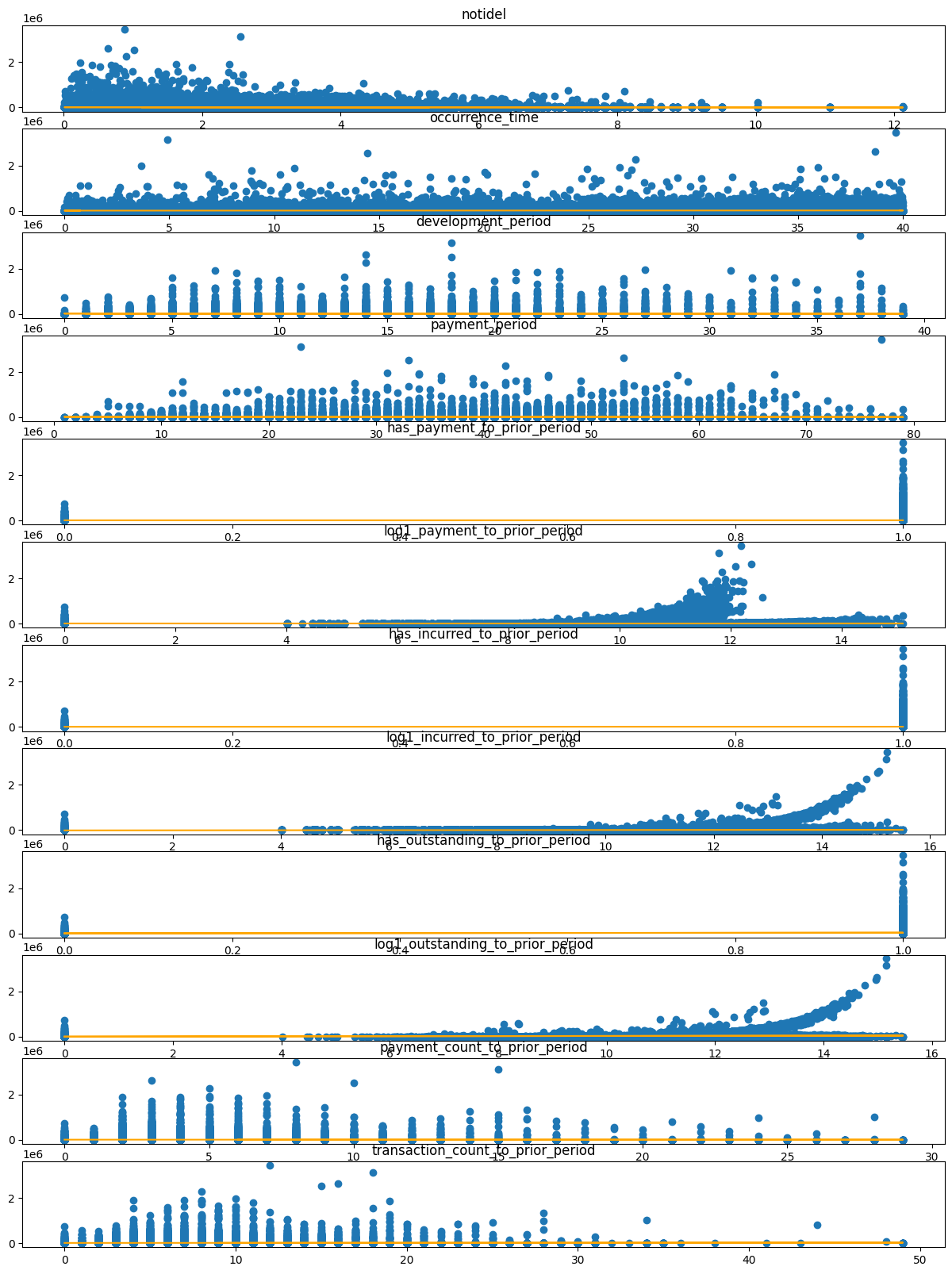

Results are very noisy, so look at data with features in a decile format:

fig, axs = plt.subplots(len(data_cols), sharex=False, sharey=True, figsize=(7, 40))

for i, f in enumerate(data_cols):
    dat_copy = dat.copy()
    dat_copy["decile"] = pd.qcut(dat[f], 10, labels=False, duplicates='drop')
    X_sum = dat_copy.groupby("decile").agg("mean").reset_index()
    
    axs[i].scatter(X_sum.index, X_sum.payment_size)
    axs[i].set_title(f)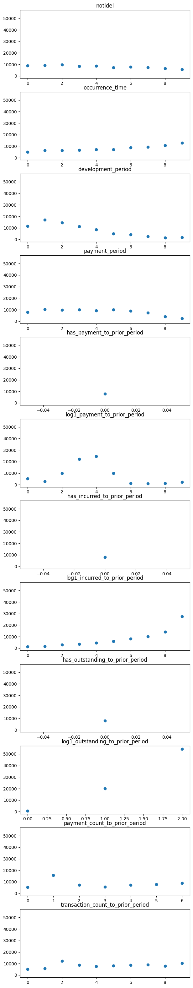

Data Augmentation

Idea: Claim information as at every balance date

Consider claim number 2000 (as an example):

sample_df = dat.loc[dat.claim_no==2000, ["claim_no", "occurrence_period", "train_ind", "payment_size"] + data_cols]
sample_df

	claim_no	occurrence_period	train_ind	payment_size	notidel	occurrence_time	development_period	payment_period	has_payment_to_prior_period	log1_payment_to_prior_period	has_incurred_to_prior_period	log1_incurred_to_prior_period	has_outstanding_to_prior_period	log1_outstanding_to_prior_period	payment_count_to_prior_period	transaction_count_to_prior_period
79961	2000	22	True	0.00	1.69	21.23	1	23	0	0.00	0	0.00	0	0.00	0.00	0.00
79962	2000	22	True	0.00	1.69	21.23	2	24	0	0.00	1	10.46	1	10.46	0.00	1.00
79963	2000	22	True	12,924.67	1.69	21.23	3	25	0	0.00	1	10.46	1	10.46	0.00	1.00
79964	2000	22	True	0.00	1.69	21.23	4	26	1	9.47	1	10.72	1	10.38	1.00	2.00
79965	2000	22	True	0.00	1.69	21.23	5	27	1	9.47	1	10.72	1	10.38	1.00	2.00
79966	2000	22	True	0.00	1.69	21.23	6	28	1	9.47	1	10.72	1	10.38	1.00	2.00
79967	2000	22	True	14,697.76	1.69	21.23	7	29	1	9.47	1	10.93	1	10.67	1.00	3.00
79968	2000	22	True	0.00	1.69	21.23	8	30	1	10.23	1	10.93	1	10.25	2.00	4.00
79969	2000	22	True	13,963.72	1.69	21.23	9	31	1	10.23	1	10.94	1	10.27	2.00	5.00
79970	2000	22	True	0.00	1.69	21.23	10	32	1	10.64	1	10.94	1	9.61	3.00	6.00
79971	2000	22	True	0.00	1.69	21.23	11	33	1	10.64	1	10.94	1	9.61	3.00	6.00
79972	2000	22	True	0.00	1.69	21.23	12	34	1	10.64	1	10.94	1	9.61	3.00	6.00
79973	2000	22	True	14,848.13	1.69	21.23	13	35	1	10.64	1	10.94	1	9.61	3.00	6.00
79974	2000	22	True	0.00	1.69	21.23	14	36	1	10.94	1	10.99	1	8.00	4.00	7.00
79975	2000	22	True	0.00	1.69	21.23	15	37	1	10.94	1	12.49	1	12.25	4.00	8.00
79976	2000	22	True	15,405.11	1.69	21.23	16	38	1	10.94	1	12.49	1	12.25	4.00	8.00
79977	2000	22	True	0.00	1.69	21.23	17	39	1	11.18	1	12.36	1	12.00	5.00	9.00
79978	2000	22	True	0.00	1.69	21.23	18	40	1	11.18	1	12.33	1	11.95	5.00	10.00
79979	2000	22	False	460,153.69	1.69	21.23	19	41	1	11.18	1	13.29	1	13.16	5.00	11.00
79980	2000	22	False	0.00	1.69	21.23	20	42	1	13.18	1	13.29	1	10.95	6.00	12.00
79981	2000	22	False	57,363.51	1.69	21.23	21	43	1	13.18	1	13.29	1	10.96	6.00	13.00
79982	2000	22	False	0.00	1.69	21.23	22	44	1	13.29	1	13.29	0	0.00	7.00	14.00
79983	2000	22	False	0.00	1.69	21.23	23	45	1	13.29	1	13.29	0	0.00	7.00	14.00
79984	2000	22	False	0.00	1.69	21.23	24	46	1	13.29	1	13.29	0	0.00	7.00	14.00
79985	2000	22	False	0.00	1.69	21.23	25	47	1	13.29	1	13.29	0	0.00	7.00	14.00
79986	2000	22	False	0.00	1.69	21.23	26	48	1	13.29	1	13.29	0	0.00	7.00	14.00
79987	2000	22	False	0.00	1.69	21.23	27	49	1	13.29	1	13.29	0	0.00	7.00	14.00
79988	2000	22	False	0.00	1.69	21.23	28	50	1	13.29	1	13.29	0	0.00	7.00	14.00
79989	2000	22	False	0.00	1.69	21.23	29	51	1	13.29	1	13.29	0	0.00	7.00	14.00
79990	2000	22	False	0.00	1.69	21.23	30	52	1	13.29	1	13.29	0	0.00	7.00	14.00
79991	2000	22	False	0.00	1.69	21.23	31	53	1	13.29	1	13.29	0	0.00	7.00	14.00
79992	2000	22	False	0.00	1.69	21.23	32	54	1	13.29	1	13.29	0	0.00	7.00	14.00
79993	2000	22	False	0.00	1.69	21.23	33	55	1	13.29	1	13.29	0	0.00	7.00	14.00
79994	2000	22	False	0.00	1.69	21.23	34	56	1	13.29	1	13.29	0	0.00	7.00	14.00
79995	2000	22	False	0.00	1.69	21.23	35	57	1	13.29	1	13.29	0	0.00	7.00	14.00
79996	2000	22	False	0.00	1.69	21.23	36	58	1	13.29	1	13.29	0	0.00	7.00	14.00
79997	2000	22	False	0.00	1.69	21.23	37	59	1	13.29	1	13.29	0	0.00	7.00	14.00
79998	2000	22	False	0.00	1.69	21.23	38	60	1	13.29	1	13.29	0	0.00	7.00	14.00
79999	2000	22	False	0.00	1.69	21.23	39	61	1	13.29	1	13.29	0	0.00	7.00	14.00

Each record represents one development period. The features are based on the history up to the development period, so at every point, we are predicting the next payment without using any future information.

However, this is any future information relative to the period. The challenge is that actuarial models are often used to predict ultimate claims, not just for the following period. Consequently, we need to predict the future payments based on information up to some date.

def backdate(df, backdate_periods, keep_cols):
    dedupe = [*set(["claim_no", "occurrence_period", "development_period", "payment_period"] + keep_cols)]
    bd = df.loc[:, dedupe].copy()
    bd["development_period"]= bd.development_period + backdate_periods
    bd.rename(columns={"payment_period": "payment_period_as_at"}, inplace=True)
    df= df[["claim_no", "occurrence_period", "development_period", "train_ind", "payment_size", "payment_period", "occurrence_time", "notidel"]].assign(
        data_as_at_development_period = lambda df: df.development_period - backdate_periods, 
        backdate_periods = backdate_periods
    ).merge(
        bd,
        how='left',
        on=["claim_no", "occurrence_period", "development_period"],
        suffixes=[None, "_backdatedrop"]
    )
    return df.drop(df.filter(regex='_backdatedrop').columns, axis=1)

backdate(sample_df, backdate_periods=1, keep_cols=data_cols)

	claim_no	occurrence_period	development_period	train_ind	payment_size	payment_period	occurrence_time	notidel	data_as_at_development_period	backdate_periods	log1_outstanding_to_prior_period	log1_payment_to_prior_period	has_incurred_to_prior_period	payment_period_as_at	has_payment_to_prior_period	has_outstanding_to_prior_period	transaction_count_to_prior_period	payment_count_to_prior_period	log1_incurred_to_prior_period
0	2000	22	1	True	0.00	23	21.23	1.69	0	1	NaN	NaN	NaN	NaN	NaN	NaN	NaN	NaN	NaN
1	2000	22	2	True	0.00	24	21.23	1.69	1	1	0.00	0.00	0.00	23.00	0.00	0.00	0.00	0.00	0.00
2	2000	22	3	True	12,924.67	25	21.23	1.69	2	1	10.46	0.00	1.00	24.00	0.00	1.00	1.00	0.00	10.46
3	2000	22	4	True	0.00	26	21.23	1.69	3	1	10.46	0.00	1.00	25.00	0.00	1.00	1.00	0.00	10.46
4	2000	22	5	True	0.00	27	21.23	1.69	4	1	10.38	9.47	1.00	26.00	1.00	1.00	2.00	1.00	10.72
5	2000	22	6	True	0.00	28	21.23	1.69	5	1	10.38	9.47	1.00	27.00	1.00	1.00	2.00	1.00	10.72
6	2000	22	7	True	14,697.76	29	21.23	1.69	6	1	10.38	9.47	1.00	28.00	1.00	1.00	2.00	1.00	10.72
7	2000	22	8	True	0.00	30	21.23	1.69	7	1	10.67	9.47	1.00	29.00	1.00	1.00	3.00	1.00	10.93
8	2000	22	9	True	13,963.72	31	21.23	1.69	8	1	10.25	10.23	1.00	30.00	1.00	1.00	4.00	2.00	10.93
9	2000	22	10	True	0.00	32	21.23	1.69	9	1	10.27	10.23	1.00	31.00	1.00	1.00	5.00	2.00	10.94
10	2000	22	11	True	0.00	33	21.23	1.69	10	1	9.61	10.64	1.00	32.00	1.00	1.00	6.00	3.00	10.94
11	2000	22	12	True	0.00	34	21.23	1.69	11	1	9.61	10.64	1.00	33.00	1.00	1.00	6.00	3.00	10.94
12	2000	22	13	True	14,848.13	35	21.23	1.69	12	1	9.61	10.64	1.00	34.00	1.00	1.00	6.00	3.00	10.94
13	2000	22	14	True	0.00	36	21.23	1.69	13	1	9.61	10.64	1.00	35.00	1.00	1.00	6.00	3.00	10.94
14	2000	22	15	True	0.00	37	21.23	1.69	14	1	8.00	10.94	1.00	36.00	1.00	1.00	7.00	4.00	10.99
15	2000	22	16	True	15,405.11	38	21.23	1.69	15	1	12.25	10.94	1.00	37.00	1.00	1.00	8.00	4.00	12.49
16	2000	22	17	True	0.00	39	21.23	1.69	16	1	12.25	10.94	1.00	38.00	1.00	1.00	8.00	4.00	12.49
17	2000	22	18	True	0.00	40	21.23	1.69	17	1	12.00	11.18	1.00	39.00	1.00	1.00	9.00	5.00	12.36
18	2000	22	19	False	460,153.69	41	21.23	1.69	18	1	11.95	11.18	1.00	40.00	1.00	1.00	10.00	5.00	12.33
19	2000	22	20	False	0.00	42	21.23	1.69	19	1	13.16	11.18	1.00	41.00	1.00	1.00	11.00	5.00	13.29
20	2000	22	21	False	57,363.51	43	21.23	1.69	20	1	10.95	13.18	1.00	42.00	1.00	1.00	12.00	6.00	13.29
21	2000	22	22	False	0.00	44	21.23	1.69	21	1	10.96	13.18	1.00	43.00	1.00	1.00	13.00	6.00	13.29
22	2000	22	23	False	0.00	45	21.23	1.69	22	1	0.00	13.29	1.00	44.00	1.00	0.00	14.00	7.00	13.29
23	2000	22	24	False	0.00	46	21.23	1.69	23	1	0.00	13.29	1.00	45.00	1.00	0.00	14.00	7.00	13.29
24	2000	22	25	False	0.00	47	21.23	1.69	24	1	0.00	13.29	1.00	46.00	1.00	0.00	14.00	7.00	13.29
25	2000	22	26	False	0.00	48	21.23	1.69	25	1	0.00	13.29	1.00	47.00	1.00	0.00	14.00	7.00	13.29
26	2000	22	27	False	0.00	49	21.23	1.69	26	1	0.00	13.29	1.00	48.00	1.00	0.00	14.00	7.00	13.29
27	2000	22	28	False	0.00	50	21.23	1.69	27	1	0.00	13.29	1.00	49.00	1.00	0.00	14.00	7.00	13.29
28	2000	22	29	False	0.00	51	21.23	1.69	28	1	0.00	13.29	1.00	50.00	1.00	0.00	14.00	7.00	13.29
29	2000	22	30	False	0.00	52	21.23	1.69	29	1	0.00	13.29	1.00	51.00	1.00	0.00	14.00	7.00	13.29
30	2000	22	31	False	0.00	53	21.23	1.69	30	1	0.00	13.29	1.00	52.00	1.00	0.00	14.00	7.00	13.29
31	2000	22	32	False	0.00	54	21.23	1.69	31	1	0.00	13.29	1.00	53.00	1.00	0.00	14.00	7.00	13.29
32	2000	22	33	False	0.00	55	21.23	1.69	32	1	0.00	13.29	1.00	54.00	1.00	0.00	14.00	7.00	13.29
33	2000	22	34	False	0.00	56	21.23	1.69	33	1	0.00	13.29	1.00	55.00	1.00	0.00	14.00	7.00	13.29
34	2000	22	35	False	0.00	57	21.23	1.69	34	1	0.00	13.29	1.00	56.00	1.00	0.00	14.00	7.00	13.29
35	2000	22	36	False	0.00	58	21.23	1.69	35	1	0.00	13.29	1.00	57.00	1.00	0.00	14.00	7.00	13.29
36	2000	22	37	False	0.00	59	21.23	1.69	36	1	0.00	13.29	1.00	58.00	1.00	0.00	14.00	7.00	13.29
37	2000	22	38	False	0.00	60	21.23	1.69	37	1	0.00	13.29	1.00	59.00	1.00	0.00	14.00	7.00	13.29
38	2000	22	39	False	0.00	61	21.23	1.69	38	1	0.00	13.29	1.00	60.00	1.00	0.00	14.00	7.00	13.29

Idea: Pinning the Tail

So one challenge with the deep learning models is the tail.

We would have an assumption that claims will generally tail off to zero in later development periods and eventually all be settled.

The training data see claims tailing off to zero, but only for the early occurrence months. With the payment period cut-off, we have no tail data for more recent occurrence months.

This is not a problem for the GLM which is parametrized to have the development period effect across all occurrence periods, but for more complex models like the neural networks it’s possible for the model to extrapolate the tail wildly.

The proposed solution below is to augment the data with tail development periods with zero payments.

extra_data = (
    dat.loc[dat.train_ind == 1, [*set(["claim_no", "occurrence_period", "development_period", "payment_period", "train_ind"] + data_cols)]]  # Training data
        .groupby("claim_no").last()  # Last training record per claim
        .rename(columns={"payment_period": "payment_period_as_at", "development_period": "data_as_at_development_period"})
        .assign(
            development_period = num_dev_periods + 1,  # set dev period to be tail
            payment_period = lambda df: df.occurrence_period + num_dev_periods + 1,
            backdate_periods = lambda df: num_dev_periods + 1 - df.payment_period,
            payment_size = 0
        )
        .reset_index()
)
extra_data.head()

	claim_no	data_as_at_development_period	log1_outstanding_to_prior_period	log1_payment_to_prior_period	has_incurred_to_prior_period	payment_period_as_at	has_payment_to_prior_period	has_outstanding_to_prior_period	log1_incurred_to_prior_period	transaction_count_to_prior_period	payment_count_to_prior_period	occurrence_time	occurrence_period	notidel	train_ind	development_period	payment_period	backdate_periods	payment_size
0	1	39	0.00	12.50	1	40	1	0	12.50	9.00	5.00	0.73	1	1.13	True	40	41	-1	0
1	2	39	0.00	12.50	1	40	1	0	12.50	9.00	5.00	0.33	1	1.26	True	40	41	-1	0
2	3	39	0.00	11.72	1	40	1	0	11.72	9.00	6.00	0.52	1	1.86	True	40	41	-1	0
3	4	39	0.00	12.41	1	40	1	0	12.41	8.00	5.00	0.74	1	0.72	True	40	41	-1	0
4	5	39	0.00	11.91	1	40	1	0	11.91	8.00	5.00	0.62	1	3.18	True	40	41	-1	0

The dataset gets quite large with the backdating, as we repeat each claim development_period squared times.

We will create a nn_train that samples one record from each claim_no, development_period.

backdated_data = [backdate(dat, backdate_periods=i, keep_cols=data_cols) for i in range(0, num_dev_periods)]
all_data = pd.concat(backdated_data + [extra_data], axis="rows")

a = set(all_data.columns.to_list())
b = set(extra_data.columns.to_list())

assert list(b - a) == []
assert list(a - b) == []

nn_train_full = all_data.loc[all_data.train_ind == 1].loc[lambda df: ~np.isnan(df.payment_period_as_at)]        # Filter out invalid payment period as at
nn_test = all_data.loc[all_data.train_ind == 0].loc[lambda df: df.payment_period_as_at==(cutoff + 1)].fillna(0)       # As at balance date
features = data_cols + ["backdate_periods"]

nn_train = nn_train_full.groupby(["claim_no", "development_period"]).sample(n=1, random_state=42)
nn_train.index.size == dat[dat.train_ind==1].index.size

nn_dat = pd.concat([nn_train.assign(train_ind=True), nn_test.assign(train_ind=False)])
# Run below instead to not use these ideas for now:
# nn_train = dat.loc[dat.train_ind == 1]
# nn_test = dat.loc[dat.train_ind == 0]

features = data_cols + ["backdate_periods"]

A more sophisticated approach could be to sample different records per epoch. We create a batch sampling function to use in our training loop.

def claim_sampler(X, y):
    indices = torch.tensor(
        nn_train_full[["claim_no", "development_period", "data_as_at_development_period"]]
        .reset_index()
        .groupby(["claim_no", "development_period"])
        .sample(n=1)
        .index
    )
    return torch.index_select(X, 0, indices), torch.index_select(y, 0, indices)

use_batching_logic=True  # Set to False to omit this logic.

nn_train_full.loc[lambda df: df.claim_no == 2000].sort_values(["development_period", "data_as_at_development_period"])

	claim_no	occurrence_period	development_period	train_ind	payment_size	payment_period	occurrence_time	notidel	data_as_at_development_period	backdate_periods	log1_outstanding_to_prior_period	log1_payment_to_prior_period	has_incurred_to_prior_period	payment_period_as_at	has_payment_to_prior_period	has_outstanding_to_prior_period	transaction_count_to_prior_period	payment_count_to_prior_period	log1_incurred_to_prior_period
75716	2000	22	1	True	0.00	23	21.23	1.69	1	0	0.00	0.00	0.00	23.00	0.00	0.00	0.00	0.00	0.00
75717	2000	22	2	True	0.00	24	21.23	1.69	1	1	0.00	0.00	0.00	23.00	0.00	0.00	0.00	0.00	0.00
75717	2000	22	2	True	0.00	24	21.23	1.69	2	0	10.46	0.00	1.00	24.00	0.00	1.00	1.00	0.00	10.46
75718	2000	22	3	True	12,924.67	25	21.23	1.69	1	2	0.00	0.00	0.00	23.00	0.00	0.00	0.00	0.00	0.00
75718	2000	22	3	True	12,924.67	25	21.23	1.69	2	1	10.46	0.00	1.00	24.00	0.00	1.00	1.00	0.00	10.46
...	...	...	...	...	...	...	...	...	...	...	...	...	...	...	...	...	...	...	...
75733	2000	22	18	True	0.00	40	21.23	1.69	15	3	12.25	10.94	1.00	37.00	1.00	1.00	8.00	4.00	12.49
75733	2000	22	18	True	0.00	40	21.23	1.69	16	2	12.25	10.94	1.00	38.00	1.00	1.00	8.00	4.00	12.49
75733	2000	22	18	True	0.00	40	21.23	1.69	17	1	12.00	11.18	1.00	39.00	1.00	1.00	9.00	5.00	12.36
75733	2000	22	18	True	0.00	40	21.23	1.69	18	0	11.95	11.18	1.00	40.00	1.00	1.00	10.00	5.00	12.33
1999	2000	22	40	True	0.00	62	21.23	1.69	18	-22	11.95	11.18	1.00	40.00	1.00	1.00	10.00	5.00	12.33

172 rows × 19 columns

nn_test.loc[lambda df: df.claim_no == 2000]

	claim_no	occurrence_period	development_period	train_ind	payment_size	payment_period	occurrence_time	notidel	data_as_at_development_period	backdate_periods	log1_outstanding_to_prior_period	log1_payment_to_prior_period	has_incurred_to_prior_period	payment_period_as_at	has_payment_to_prior_period	has_outstanding_to_prior_period	transaction_count_to_prior_period	payment_count_to_prior_period	log1_incurred_to_prior_period
75734	2000	22	19	False	460,153.69	41	21.23	1.69	19	0	13.16	11.18	1.00	41.00	1.00	1.00	11.00	5.00	13.29
75735	2000	22	20	False	0.00	42	21.23	1.69	19	1	13.16	11.18	1.00	41.00	1.00	1.00	11.00	5.00	13.29
75736	2000	22	21	False	57,363.51	43	21.23	1.69	19	2	13.16	11.18	1.00	41.00	1.00	1.00	11.00	5.00	13.29
75737	2000	22	22	False	0.00	44	21.23	1.69	19	3	13.16	11.18	1.00	41.00	1.00	1.00	11.00	5.00	13.29
75738	2000	22	23	False	0.00	45	21.23	1.69	19	4	13.16	11.18	1.00	41.00	1.00	1.00	11.00	5.00	13.29
75739	2000	22	24	False	0.00	46	21.23	1.69	19	5	13.16	11.18	1.00	41.00	1.00	1.00	11.00	5.00	13.29
75740	2000	22	25	False	0.00	47	21.23	1.69	19	6	13.16	11.18	1.00	41.00	1.00	1.00	11.00	5.00	13.29
75741	2000	22	26	False	0.00	48	21.23	1.69	19	7	13.16	11.18	1.00	41.00	1.00	1.00	11.00	5.00	13.29
75742	2000	22	27	False	0.00	49	21.23	1.69	19	8	13.16	11.18	1.00	41.00	1.00	1.00	11.00	5.00	13.29
75743	2000	22	28	False	0.00	50	21.23	1.69	19	9	13.16	11.18	1.00	41.00	1.00	1.00	11.00	5.00	13.29
75744	2000	22	29	False	0.00	51	21.23	1.69	19	10	13.16	11.18	1.00	41.00	1.00	1.00	11.00	5.00	13.29
75745	2000	22	30	False	0.00	52	21.23	1.69	19	11	13.16	11.18	1.00	41.00	1.00	1.00	11.00	5.00	13.29
75746	2000	22	31	False	0.00	53	21.23	1.69	19	12	13.16	11.18	1.00	41.00	1.00	1.00	11.00	5.00	13.29
75747	2000	22	32	False	0.00	54	21.23	1.69	19	13	13.16	11.18	1.00	41.00	1.00	1.00	11.00	5.00	13.29
75748	2000	22	33	False	0.00	55	21.23	1.69	19	14	13.16	11.18	1.00	41.00	1.00	1.00	11.00	5.00	13.29
75749	2000	22	34	False	0.00	56	21.23	1.69	19	15	13.16	11.18	1.00	41.00	1.00	1.00	11.00	5.00	13.29
75750	2000	22	35	False	0.00	57	21.23	1.69	19	16	13.16	11.18	1.00	41.00	1.00	1.00	11.00	5.00	13.29
75751	2000	22	36	False	0.00	58	21.23	1.69	19	17	13.16	11.18	1.00	41.00	1.00	1.00	11.00	5.00	13.29
75752	2000	22	37	False	0.00	59	21.23	1.69	19	18	13.16	11.18	1.00	41.00	1.00	1.00	11.00	5.00	13.29
75753	2000	22	38	False	0.00	60	21.23	1.69	19	19	13.16	11.18	1.00	41.00	1.00	1.00	11.00	5.00	13.29
75754	2000	22	39	False	0.00	61	21.23	1.69	19	20	13.16	11.18	1.00	41.00	1.00	1.00	11.00	5.00	13.29

nn_test.loc[nn_test.occurrence_period==40]

	claim_no	occurrence_period	development_period	train_ind	payment_size	payment_period	occurrence_time	notidel	data_as_at_development_period	backdate_periods	log1_outstanding_to_prior_period	log1_payment_to_prior_period	has_incurred_to_prior_period	payment_period_as_at	has_payment_to_prior_period	has_outstanding_to_prior_period	transaction_count_to_prior_period	payment_count_to_prior_period	log1_incurred_to_prior_period
135553	3582	40	1	False	0.00	41	39.26	0.22	1	0	10.53	0.00	1.00	41.00	0.00	1.00	1.00	0.00	10.53
135630	3584	40	1	False	0.00	41	39.29	1.48	1	0	0.00	0.00	0.00	41.00	0.00	0.00	0.00	0.00	0.00
135707	3586	40	1	False	32,340.10	41	39.95	0.28	1	0	0.00	0.00	0.00	41.00	0.00	0.00	0.00	0.00	0.00
135781	3588	40	1	False	0.00	41	39.67	0.87	1	0	0.00	0.00	0.00	41.00	0.00	0.00	0.00	0.00	0.00
135820	3589	40	1	False	0.00	41	39.94	0.27	1	0	0.00	0.00	0.00	41.00	0.00	0.00	0.00	0.00	0.00
...	...	...	...	...	...	...	...	...	...	...	...	...	...	...	...	...	...	...	...
138157	3650	40	39	False	0.00	79	39.31	0.22	1	38	9.59	0.00	1.00	41.00	0.00	1.00	1.00	0.00	9.59
138344	3655	40	39	False	0.00	79	39.14	1.64	1	38	0.00	0.00	0.00	41.00	0.00	0.00	0.00	0.00	0.00
138494	3659	40	39	False	0.00	79	39.54	0.16	1	38	12.63	0.00	1.00	41.00	0.00	1.00	1.00	0.00	12.63
138534	3660	40	39	False	0.00	79	39.43	0.51	1	38	13.08	0.00	1.00	41.00	0.00	1.00	1.00	0.00	13.08
138574	3661	40	39	False	0.00	79	39.36	0.46	1	38	11.11	0.00	1.00	41.00	0.00	1.00	1.00	0.00	11.11

1209 rows × 19 columns

dat.loc[dat.occurrence_period==40, nn_test.columns]

	claim_no	occurrence_period	development_period	train_ind	payment_size	payment_period	occurrence_time	notidel	data_as_at_development_period	backdate_periods	log1_outstanding_to_prior_period	log1_payment_to_prior_period	has_incurred_to_prior_period	payment_period_as_at	has_payment_to_prior_period	has_outstanding_to_prior_period	transaction_count_to_prior_period	payment_count_to_prior_period	log1_incurred_to_prior_period
143240	3582	40	0	True	0.00	40	39.26	0.22	0	0	0.00	0.00	0	40	0	0	0.00	0.00	0.00
143241	3582	40	1	False	0.00	41	39.26	0.22	1	0	10.53	0.00	1	41	0	1	1.00	0.00	10.53
143242	3582	40	2	False	15,226.59	42	39.26	0.22	2	0	10.53	0.00	1	42	0	1	1.00	0.00	10.53
143243	3582	40	3	False	0.00	43	39.26	0.22	3	0	10.43	9.63	1	43	1	1	2.00	1.00	10.80
143244	3582	40	4	False	16,196.52	44	39.26	0.22	4	0	10.43	9.63	1	44	1	1	2.00	1.00	10.80
...	...	...	...	...	...	...	...	...	...	...	...	...	...	...	...	...	...	...	...
146515	3663	40	35	False	0.00	75	39.87	5.27	35	0	0.00	13.61	1	75	1	0	9.00	6.00	13.61
146516	3663	40	36	False	0.00	76	39.87	5.27	36	0	0.00	13.61	1	76	1	0	9.00	6.00	13.61
146517	3663	40	37	False	0.00	77	39.87	5.27	37	0	0.00	13.61	1	77	1	0	9.00	6.00	13.61
146518	3663	40	38	False	0.00	78	39.87	5.27	38	0	0.00	13.61	1	78	1	0	9.00	6.00	13.61
146519	3663	40	39	False	0.00	79	39.87	5.27	39	0	0.00	13.61	1	79	1	0	9.00	6.00	13.61

3092 rows × 19 columns

Detailed Neural Network

This logic follows a similar pipeline to the basic neural network but including the features.

SplineNet:

model_resnet_detailed = Pipeline(
    steps=[
        ("keep", ColumnKeeper(features)),  
        ('zero_to_one', MinMaxScaler()),       # Important! Standardize deep learning inputs.
        ("model", RandomizedSearchCV(
            TabularNetRegressor(LogLinkResNet),
            parameters_nn,
            n_jobs=4,  # Run in parallel (small model)
            n_iter=cv_runs, # Models train slowly, so try only a few models
            cv=RollingOriginSplit(5,5).split(groups=nn_train.payment_period),
            random_state=42
        )),
    ]
)

model_resnet_detailed.fit(
    nn_train,
    nn_train.loc[:, ["payment_size"]]
)

bst_res_det = model_resnet_detailed["model"].best_params_
print("best parameters:", bst_res_det)

cv_results_res_detailed = pd.DataFrame(model_resnet_detailed["model"].cv_results_)


# Refit best model for longer iters
model_resnet_detailed = Pipeline(
    steps=[
        ("keep", ColumnKeeper(features)),  
        ('zero_to_one', MinMaxScaler()),       # Important! Standardize deep learning inputs.
        ("model", TabularNetRegressor(
                SplineNet, 
                l1_penalty=bst_res_det["l1_penalty"],
                weight_decay=bst_res_det["weight_decay"],  
                n_hidden=bst_res_det["n_hidden"],   
                dropout=bst_res_det["dropout"],                             
                max_iter=nn_iter, 
                max_lr=bst_res_det["max_lr"],                
                batch_function=claim_sampler if use_batching_logic else None,                
                rebatch_every_iter=mdn_iter/10,  # takes over 1s to resample so iterate a few epochs per resample                
            )
        )
    ]
)

if use_batching_logic:
    model_resnet_detailed.fit(
        nn_train_full,
        nn_train_full.loc[:, ["payment_size"]]
    )
else: 
    model_resnet_detailed.fit(
        nn_train,
        nn_train.loc[:, ["payment_size"]]
    )

best parameters: {'weight_decay': 0.01, 'verbose': 0, 'n_hidden': 10, 'max_lr': 0.05, 'max_iter': 100, 'l1_penalty': 0.0, 'keep_best_model': True, 'dropout': 0.5, 'clip_value': None}
Train RMSE:  54727.0859375  Train Loss:  -72119.28125
refreshing batch on epoch 0
Train RMSE:  54085.41796875  Train Loss:  -76427.2890625
refreshing batch on epoch 50
Train RMSE:  54353.5859375  Train Loss:  -77095.7421875
refreshing batch on epoch 100
Train RMSE:  53831.265625  Train Loss:  -77777.6484375
refreshing batch on epoch 150
Train RMSE:  53840.56640625  Train Loss:  -77741.328125
refreshing batch on epoch 200
Train RMSE:  53813.30078125  Train Loss:  -77861.6484375
refreshing batch on epoch 250
Train RMSE:  53815.609375  Train Loss:  -77779.140625
refreshing batch on epoch 300
Train RMSE:  53772.734375  Train Loss:  -78098.1171875
refreshing batch on epoch 350
Train RMSE:  53779.421875  Train Loss:  -78083.203125
refreshing batch on epoch 400
Train RMSE:  53768.2265625  Train Loss:  -78098.3671875
refreshing batch on epoch 450

make_model_subplots(model_resnet_detailed, dat)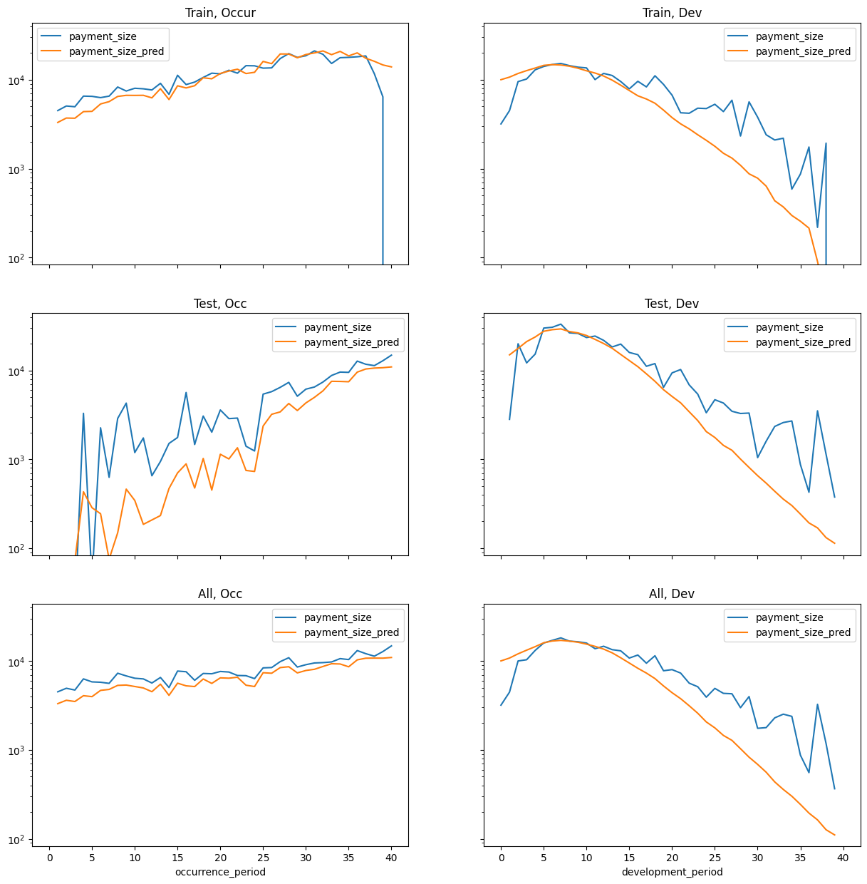

make_model_subplots(model_resnet_detailed, nn_dat)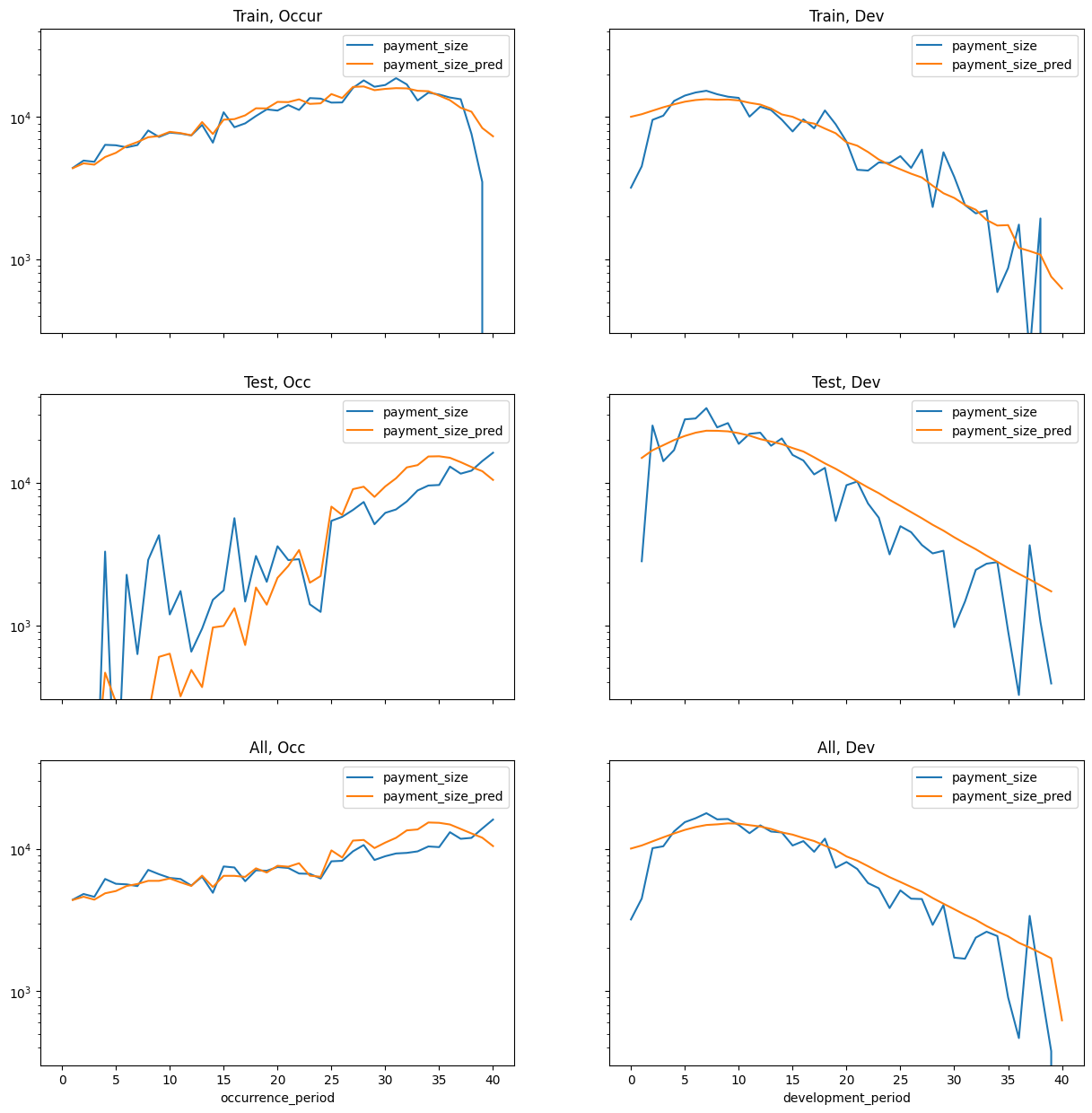

dat_resnet_det_pred, triangle_resnet_detailed = make_pred_set_and_triangle(model_resnet_detailed, nn_train, nn_test)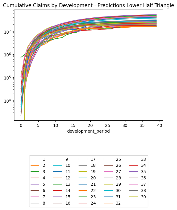

dat["pred_resnet_claims"] = model_resnet_detailed.predict(dat)
dat["pred_resnet_claims_decile"] = pd.qcut(dat["pred_resnet_claims"], 10, labels=False, duplicates='drop')

# Train only
X_sum = dat.loc[dat.train_ind == 1].groupby("pred_resnet_claims_decile").agg("mean").reset_index()

X_sum = dat.groupby("pred_resnet_claims_decile").agg("mean").reset_index()

plt.scatter(X_sum.pred_resnet_claims, X_sum.payment_size)
m = max(X_sum.pred_resnet_claims.max(), X_sum.payment_size.max())
plt.plot([0, m],[0, m])

# Test only
X_sum = dat.loc[dat.train_ind == 0].groupby("pred_resnet_claims_decile").agg("mean").reset_index()

plt.scatter(X_sum.pred_resnet_claims, X_sum.payment_size)
m = max(X_sum.pred_resnet_claims.max(), X_sum.payment_size.max())

plt.plot([0, m],[0, m])

SplineNet:

model_splinenet_detailed = Pipeline(
    steps=[
        ("keep", ColumnKeeper(features)),  
        ('zero_to_one', MinMaxScaler()),       # Important! Standardize deep learning inputs.
        ("model", RandomizedSearchCV(
            TabularNetRegressor(SplineNet),
            parameters_nn,
            n_jobs=4,  # Run in parallel (small model)
            n_iter=cv_runs, # Models train slowly, so try only a few models
            cv=RollingOriginSplit(5,5).split(groups=nn_train.payment_period),
            random_state=42
        )),
    ]
)

model_splinenet_detailed.fit(
    nn_train,
    nn_train.loc[:, ["payment_size"]]
)

bst_det = model_splinenet_detailed["model"].best_params_
print("best parameters:", bst_det)

cv_results_detailed = pd.DataFrame(model_splinenet_detailed["model"].cv_results_)


# Refit best model for longer iters
model_splinenet_detailed = Pipeline(
    steps=[
        ("keep", ColumnKeeper(features)),  
        ('zero_to_one', MinMaxScaler()),       # Important! Standardize deep learning inputs.
        ("model", TabularNetRegressor(
                SplineNet, 
                l1_penalty=bst_det["l1_penalty"],
                weight_decay=bst_det["weight_decay"],  
                n_hidden=bst_det["n_hidden"],   
                dropout=bst_det["dropout"],                             
                max_iter=nn_iter, 
                max_lr=bst_det["max_lr"],                
                batch_function=claim_sampler if use_batching_logic else None,                
                rebatch_every_iter=mdn_iter/10,  # takes over 1s to resample so iterate a few epochs per resample                
            )
        )
    ]
)

if use_batching_logic:
    model_splinenet_detailed.fit(
        nn_train_full,
        nn_train_full.loc[:, ["payment_size"]]
    )
else: 
    model_splinenet_detailed.fit(
        nn_train,
        nn_train.loc[:, ["payment_size"]]
    )

best parameters: {'weight_decay': 0.01, 'verbose': 0, 'n_hidden': 10, 'max_lr': 0.05, 'max_iter': 100, 'l1_penalty': 0.0, 'keep_best_model': True, 'dropout': 0.5, 'clip_value': None}
Train RMSE:  54725.71484375  Train Loss:  -72119.28125
refreshing batch on epoch 0
Train RMSE:  54101.71484375  Train Loss:  -76451.703125
refreshing batch on epoch 50
Train RMSE:  53882.55859375  Train Loss:  -77524.34375
refreshing batch on epoch 100
Train RMSE:  53936.40234375  Train Loss:  -76640.3984375
refreshing batch on epoch 150
Train RMSE:  53838.6875  Train Loss:  -77731.515625
refreshing batch on epoch 200
Train RMSE:  53799.36328125  Train Loss:  -77964.8125
refreshing batch on epoch 250
Train RMSE:  53773.82421875  Train Loss:  -78052.8828125
refreshing batch on epoch 300
Train RMSE:  53774.40234375  Train Loss:  -77963.5390625
refreshing batch on epoch 350
Train RMSE:  53782.2109375  Train Loss:  -78030.90625
refreshing batch on epoch 400
Train RMSE:  53766.69921875  Train Loss:  -78186.703125
refreshing batch on epoch 450

make_model_subplots(model_splinenet_detailed, dat)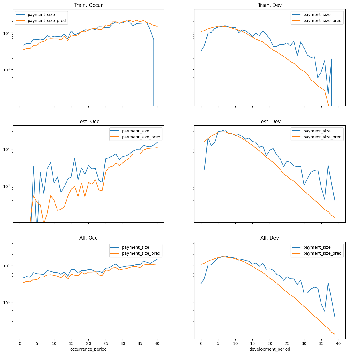

make_model_subplots(model_splinenet_detailed, nn_dat)

dat_spline_det_pred, triangle_spline_detailed = make_pred_set_and_triangle(model_splinenet_detailed, nn_train, nn_test)

dat["pred_nn_claims"] = model_splinenet_detailed.predict(dat)
dat["pred_nn_claims_decile"] = pd.qcut(dat["pred_nn_claims"], 10, labels=False, duplicates='drop')

# Train only
X_sum = dat.loc[dat.train_ind == 1].groupby("pred_nn_claims_decile").agg("mean").reset_index()

X_sum = dat.groupby("pred_nn_claims_decile").agg("mean").reset_index()

plt.scatter(X_sum.pred_nn_claims, X_sum.payment_size)
m = max(X_sum.pred_nn_claims.max(), X_sum.payment_size.max())
plt.plot([0, m],[0, m])

# Test only
X_sum = dat.loc[dat.train_ind == 0].groupby("pred_nn_claims_decile").agg("mean").reset_index()

plt.scatter(X_sum.pred_nn_claims, X_sum.payment_size)
m = max(X_sum.pred_nn_claims.max(), X_sum.payment_size.max())

plt.plot([0, m],[0, m])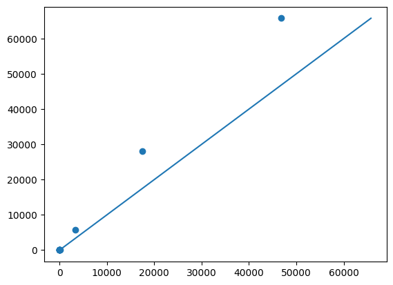

Detailed MDN

As we get to larger MDN model, the CV adds to the run-time, but based on the CV performance of the point-estimate models we are not really sure if it improves results.

So here the approach is:

• Single model run
• Add the features
• Bring across the interactions and dropout parameters from the point estimate CV
• Apply a low learn rate and clip norm for numerical stability.

model_MDN_detailed = Pipeline(
    steps=[
        ("keep", ColumnKeeper(features)),   
        ('zero_to_one', MinMaxScaler()),       # Important! Standardize deep learning inputs.
        ("model", TabularNetRegressor(
                LognormalSplineMDN, 
                n_hidden=bst_det["n_hidden"], 
                max_iter=mdn_iter, 
                max_lr=0.025,  
                # weight decay and l1 may lead to unexpected behaviour, leave it off
                dropout=bst_det["dropout"],
                n_gaussians=3,
                criterion=log_mdn_loss_fn,
                init_extra=[model_splinenet_detailed["model"].module_.state_dict(), mdn_init_bias],
                keep_best_model=True,
                # clip_value=3.0,
                batch_function=claim_sampler if use_batching_logic else None,
                rebatch_every_iter=mdn_iter/10,  # takes over 1s to resample so iterate a few epochs per resample
            )
        )
    ]
)

# Fit model
if use_batching_logic:
    model_MDN_detailed.fit(
        nn_train_full,
        nn_train_full.loc[:, ["payment_size"]]
    )    
else:
    model_MDN_detailed.fit(
        nn_train,
        nn_train.loc[:, ["payment_size"]]
    )

Train RMSE:  53765.6328125  Train Loss:  155.98707580566406
refreshing batch on epoch 0
Train RMSE:  53765.6328125  Train Loss:  5.832543849945068
refreshing batch on epoch 50
Train RMSE:  53765.6328125  Train Loss:  2.8419244289398193
refreshing batch on epoch 100
Train RMSE:  53765.6328125  Train Loss:  2.398144006729126
refreshing batch on epoch 150
Train RMSE:  53765.6328125  Train Loss:  2.3014259338378906
refreshing batch on epoch 200
Train RMSE:  53765.6328125  Train Loss:  2.2549655437469482
refreshing batch on epoch 250
Train RMSE:  53765.6328125  Train Loss:  2.219618797302246
refreshing batch on epoch 300
Train RMSE:  53765.6328125  Train Loss:  2.192033290863037
refreshing batch on epoch 350
Train RMSE:  53765.6328125  Train Loss:  2.1750428676605225
refreshing batch on epoch 400
Train RMSE:  53765.6328125  Train Loss:  2.1675562858581543
refreshing batch on epoch 450

make_model_subplots(model_MDN_detailed, dat)

make_model_subplots(model_MDN_detailed, nn_dat)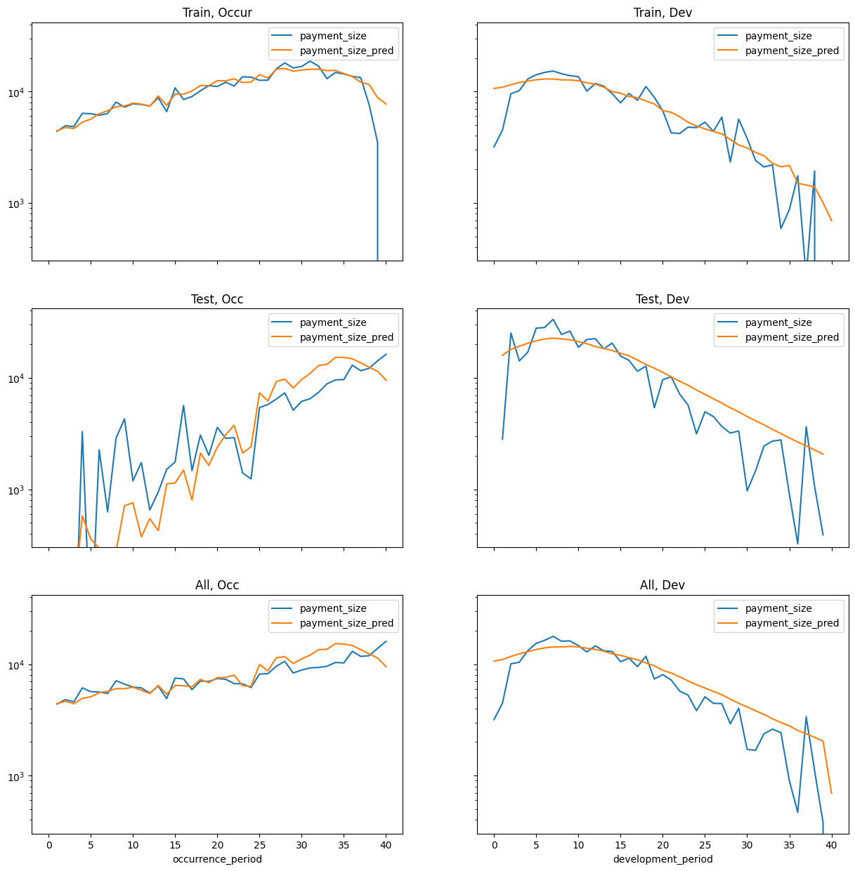

make_distribution_subplots(model_MDN_detailed)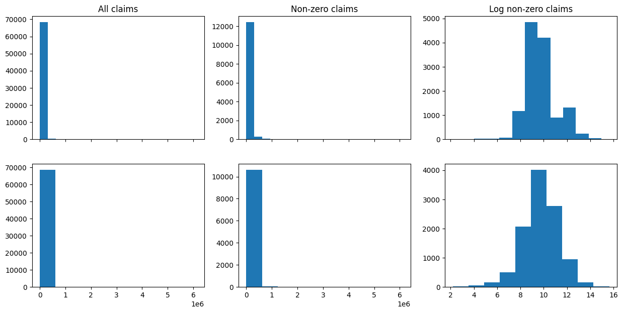

dat["pred_mdn_claims"] = model_MDN_detailed.predict(dat)
dat["pred_mdn_claims_decile"] = pd.qcut(dat["pred_mdn_claims"], 10, labels=False, duplicates='drop')

# Train only
X_sum = dat.loc[dat.train_ind == 1].groupby("pred_mdn_claims_decile").agg("mean").reset_index()

X_sum = dat.groupby("pred_mdn_claims_decile").agg("mean").reset_index()

plt.scatter(X_sum.pred_mdn_claims, X_sum.payment_size)
m = max(X_sum.pred_mdn_claims.max(), X_sum.payment_size.max())
plt.plot([0, m],[0, m])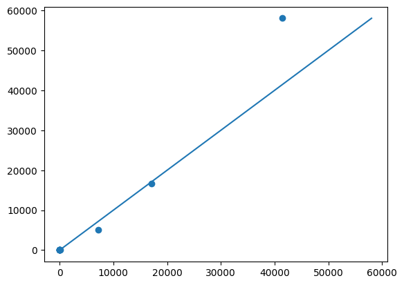

# Test only
X_sum = dat.loc[dat.train_ind == 0].groupby("pred_mdn_claims_decile").agg("mean").reset_index()

plt.scatter(X_sum.pred_mdn_claims, X_sum.payment_size)
m = max(X_sum.pred_mdn_claims.max(), X_sum.payment_size.max())

plt.plot([0, m],[0, m])

# for later comparison
dat_mdn_pred, triangle_mdn_detailed = make_pred_set_and_triangle(model_MDN_detailed, nn_train, nn_test)

dat_mdn_pred.loc[np.abs(dat_spline_det_pred.payment_size_cumulative - dat_mdn_pred.payment_size_cumulative) > 1]

	claim_no	occurrence_period	development_period	train_ind	payment_size	payment_period	occurrence_time	notidel	data_as_at_development_period	backdate_periods	log1_outstanding_to_prior_period	log1_payment_to_prior_period	has_incurred_to_prior_period	payment_period_as_at	has_payment_to_prior_period	has_outstanding_to_prior_period	transaction_count_to_prior_period	payment_count_to_prior_period	log1_incurred_to_prior_period	payment_size_cumulative

dat_spline_det_pred.loc[lambda df: (df.claim_no == 349) & (df.train_ind == False)]

	claim_no	occurrence_period	development_period	train_ind	payment_size	payment_period	occurrence_time	notidel	data_as_at_development_period	backdate_periods	log1_outstanding_to_prior_period	log1_payment_to_prior_period	has_incurred_to_prior_period	payment_period_as_at	has_payment_to_prior_period	has_outstanding_to_prior_period	transaction_count_to_prior_period	payment_count_to_prior_period	log1_incurred_to_prior_period	payment_size_cumulative
13238	349	4	37	False	10,822.77	41	3.86	1.84	37	0	13.83	11.21	1.00	41.00	1.00	1.00	8.00	3.00	13.90	84,392.68
13239	349	4	38	False	10,290.16	42	3.86	1.84	37	1	13.83	11.21	1.00	41.00	1.00	1.00	8.00	3.00	13.90	94,682.83
13240	349	4	39	False	9,778.47	43	3.86	1.84	37	2	13.83	11.21	1.00	41.00	1.00	1.00	8.00	3.00	13.90	104,461.31

dat_mdn_pred.loc[lambda df: (df.claim_no == 349) & (df.train_ind == False)]

	claim_no	occurrence_period	development_period	train_ind	payment_size	payment_period	occurrence_time	notidel	data_as_at_development_period	backdate_periods	log1_outstanding_to_prior_period	log1_payment_to_prior_period	has_incurred_to_prior_period	payment_period_as_at	has_payment_to_prior_period	has_outstanding_to_prior_period	transaction_count_to_prior_period	payment_count_to_prior_period	log1_incurred_to_prior_period	payment_size_cumulative
13238	349	4	37	False	10,822.77	41	3.86	1.84	37	0	13.83	11.21	1.00	41.00	1.00	1.00	8.00	3.00	13.90	84,392.68
13239	349	4	38	False	10,290.16	42	3.86	1.84	37	1	13.83	11.21	1.00	41.00	1.00	1.00	8.00	3.00	13.90	94,682.83
13240	349	4	39	False	9,778.47	43	3.86	1.84	37	2	13.83	11.21	1.00	41.00	1.00	1.00	8.00	3.00	13.90	104,461.31

Gradient Boosting Individual Model

We create a GBM model to use as a baseline. Advantage of GBMs is that it is really easy to get good, reasonable results. It is unable to extrapolate wildly in unexpected ways, but the disadvantage is that it is unlikely to correctly extrapolate payment period trends. There are no payment period trends in this simulated data, so should do well:

parameters_gbm = {
    "max_iter": [500, 1000, 2000, 5000], 
    "l2_regularization": [0, 0.001, 0.01, 0.1, 0.3],
    "loss": ["poisson"], 
    "learning_rate": [0.03, 0.07, 0.1]
}

gradient_boosting = Pipeline(
    steps=[
        ("keep", ColumnKeeper(features)),         
        ('gbm', RandomizedSearchCV(
                  HistGradientBoostingRegressor(),
                  parameters_gbm,
                  n_jobs=-1, # Run in parallel
                  n_iter=cv_runs, # Models train slowly, so try only a few models
                  cv=RollingOriginSplit(5,5).split(groups=nn_train.payment_period),
                  random_state=0)),
    ]
)

gradient_boosting.fit(
    nn_train,
    nn_train.payment_size
)

print(gradient_boosting["gbm"].best_params_)

{'max_iter': 2000, 'loss': 'poisson', 'learning_rate': 0.03, 'l2_regularization': 0.01}

make_model_subplots(gradient_boosting, dat)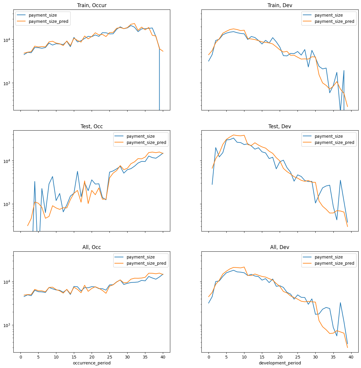

make_model_subplots(gradient_boosting, nn_dat)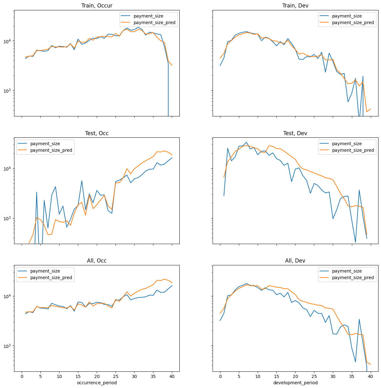

dat_gbm_pred, triangle_gbm_ind = make_pred_set_and_triangle(gradient_boosting, nn_train, nn_test)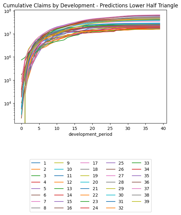

Individual Claims Predictiveness

Check how the individual models perform on train and test data.

dat["pred_gbm_claims"] = gradient_boosting.predict(dat)
dat["pred_gbm_claims_decile"] = pd.qcut(dat["pred_gbm_claims"], 10, labels=False, duplicates='drop')

# Train only
X_sum = dat.loc[dat.train_ind == 1].groupby("pred_gbm_claims_decile").agg("mean").reset_index()

X_sum = dat.groupby("pred_gbm_claims_decile").agg("mean").reset_index()

plt.scatter(X_sum.pred_gbm_claims, X_sum.payment_size)
m = max(X_sum.pred_gbm_claims.max(), X_sum.payment_size.max())
plt.plot([0, m],[0, m])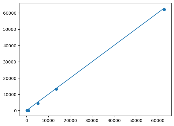

# Test only
X_sum = dat.loc[dat.train_ind == 0].groupby("pred_gbm_claims_decile").agg("mean").reset_index()

plt.scatter(X_sum.pred_gbm_claims, X_sum.payment_size)
m = max(X_sum.pred_gbm_claims.max(), X_sum.payment_size.max())
plt.plot([0, m],[0, m])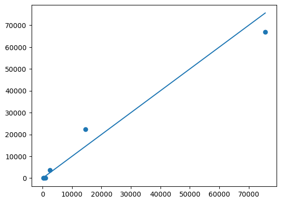

Ultimate Summary

Compare Ultimate projections from the different models

pd.options.display.float_format = '{:,.0f}'.format

results = pd.concat(
    [(
        triangle.loc[lambda df: df.payment_period == cutoff, ["occurrence_period", "payment_size_cumulative"]]
        .set_index("occurrence_period")
        .rename(columns={"payment_size_cumulative": "Paid to Date"})
    )] +
    [(df.loc[lambda df: df.development_period == num_dev_periods, ["occurrence_period", "payment_size_cumulative"]]
        .set_index("occurrence_period")
        .rename(columns={"payment_size_cumulative": l})) for df, l in zip(
            [triangle,         triangle_cl,    triangle_glm_agg,  triangle_glm_ind, triangle_spline_ind, triangle_resnet_do, triangle_nn_spline, triangle_mdn_spline, triangle_nn_cv, triangle_resnet_detailed, triangle_spline_detailed, triangle_mdn_detailed, triangle_gbm_ind],
            ["True Ultimate", "Chain Ladder", "GLM Chain Ladder", "GLM Individual", "GLM Spline",         "D/O ResNet",      "D/O SplineNet",  "D/O SplineMDN ",   "D/O SplineNet CV", "Detailed ResNet",  "Detailed SplineNet", "Detailed SplineMDN", "Detailed GBM"]
        )
    ],
    axis="columns"
).sort_index()

results

	Paid to Date	True Ultimate	Chain Ladder	GLM Chain Ladder	GLM Individual	GLM Spline	D/O ResNet	D/O SplineNet	D/O SplineMDN	D/O SplineNet CV	Detailed ResNet	Detailed SplineNet	Detailed SplineMDN	Detailed GBM
occurrence_period
1	17,485,892	17,485,892	17,485,892	17,485,892	17,485,892	17,485,892	17,485,892	17,485,892	17,485,892	17,485,892	17,485,892	17,485,892	17,485,892	17,485,892
2	15,795,103	15,795,103	15,795,103	15,795,134	15,821,221	15,866,280	15,888,352	15,906,488	15,906,488	15,888,234	15,800,222	15,801,500	15,801,500	15,821,457
3	16,108,434	16,111,727	16,285,616	16,285,647	16,312,055	16,280,810	16,322,010	16,356,091	16,356,091	16,323,868	16,121,592	16,126,862	16,126,862	16,190,916
4	18,155,534	18,935,352	18,377,934	18,377,972	18,424,706	18,410,586	18,456,274	18,493,792	18,493,792	18,461,874	18,265,570	18,292,784	18,292,784	18,396,958
5	19,235,524	19,250,872	19,653,886	19,653,922	19,710,680	19,659,068	19,713,468	19,756,592	19,756,592	19,727,088	19,337,093	19,361,392	19,361,392	19,562,238
6	21,611,440	22,786,944	22,181,350	22,181,390	22,240,392	22,307,848	22,367,292	22,409,770	22,409,770	22,396,284	21,736,698	21,765,160	21,765,160	21,985,755
7	18,526,526	18,861,376	19,072,624	19,072,656	19,132,282	19,319,268	19,357,838	19,376,774	19,376,774	19,397,918	18,608,061	18,630,599	18,630,599	18,771,394
8	27,839,500	30,036,106	28,984,746	28,984,798	29,073,758	29,090,414	29,112,122	29,099,470	29,099,470	29,186,056	28,016,788	28,051,537	28,051,537	28,195,846
9	19,798,286	22,849,618	20,828,210	20,828,248	20,893,272	21,082,996	21,071,046	21,017,720	21,017,720	21,157,624	20,225,237	20,304,972	20,304,972	20,458,580
10	23,628,224	24,720,896	25,154,980	25,155,024	25,229,162	25,445,416	25,387,422	25,258,898	25,258,898	25,524,670	24,207,924	24,322,480	24,322,480	24,405,912
11	24,596,934	26,525,608	26,682,368	26,682,414	26,753,536	27,000,192	26,877,728	26,641,880	26,641,880	27,078,678	24,948,550	25,011,901	25,011,901	25,498,735
12	15,848,811	16,394,228	17,685,404	17,685,432	17,725,470	17,822,516	17,690,942	17,446,042	17,446,042	17,872,032	16,254,583	16,304,961	16,304,961	16,587,953
13	24,036,898	25,194,832	27,142,022	27,142,064	27,220,448	27,177,784	26,929,468	26,462,016	26,462,016	27,243,664	24,487,006	24,558,175	24,558,175	24,908,239
14	17,040,986	18,981,944	19,829,872	19,829,908	19,866,636	20,619,532	20,302,944	19,686,090	19,686,090	20,691,322	18,282,593	18,478,140	18,478,140	18,637,493
15	25,963,162	28,375,866	30,920,786	30,920,842	31,070,692	30,085,996	29,692,482	28,889,976	28,889,976	30,175,932	27,319,403	27,525,937	27,525,937	28,493,595
16	19,147,944	27,107,038	23,450,766	23,450,812	23,485,770	23,717,874	23,257,828	22,272,546	22,272,546	23,834,454	21,004,365	21,249,098	21,249,098	22,053,924
17	20,473,130	22,796,338	25,722,546	25,722,592	25,791,608	26,003,652	25,423,924	24,123,716	24,123,716	26,171,146	21,622,966	21,741,627	21,741,627	22,269,693
18	18,259,918	22,533,702	23,552,468	23,552,510	23,607,782	23,501,260	22,931,582	21,606,382	21,606,382	23,685,548	20,825,912	21,201,268	21,201,268	22,299,554
19	20,525,112	23,686,100	27,099,510	27,099,558	27,161,088	26,869,550	26,152,032	24,449,804	24,449,804	27,117,410	22,708,353	23,091,859	23,091,859	22,941,089
20	23,967,498	31,330,774	32,407,678	32,407,738	32,430,768	32,939,240	31,872,852	29,356,400	29,356,400	33,305,976	28,383,144	28,863,218	28,863,218	27,752,390
21	23,882,838	29,962,468	33,551,694	33,551,760	33,740,196	33,911,348	32,639,526	29,759,118	29,759,118	34,307,548	29,412,685	30,428,752	30,428,752	28,776,498
22	18,409,002	24,089,654	27,242,720	27,242,776	27,392,162	28,433,204	27,057,726	24,183,322	24,183,322	28,779,724	24,999,340	25,750,220	25,750,220	23,957,820
23	20,920,498	23,758,476	33,155,220	33,155,284	33,319,848	32,220,078	30,529,388	27,370,516	27,370,516	32,519,086	24,946,902	25,192,274	25,192,274	24,446,417
24	18,047,780	20,501,736	30,175,460	30,175,516	30,403,008	30,080,486	28,113,480	24,897,982	24,897,982	30,270,470	22,429,679	22,805,165	22,805,165	21,000,008
25	13,656,915	23,132,220	24,360,950	24,360,996	24,405,170	25,282,098	23,211,626	20,291,212	20,291,212	25,320,104	25,585,984	26,500,339	26,500,339	22,561,164
26	14,057,512	25,597,836	26,520,252	26,520,298	26,545,318	28,534,582	25,743,200	22,373,132	22,373,132	28,385,354	25,949,932	26,467,517	26,467,517	24,389,678
27	19,192,766	34,954,040	38,892,552	38,892,628	39,134,660	38,475,344	34,486,064	30,378,120	30,378,120	38,010,264	41,257,998	41,837,961	41,837,961	34,845,121
28	20,606,538	39,625,828	45,626,804	45,626,900	45,760,488	42,853,872	37,968,644	33,677,224	33,677,224	42,023,360	44,954,913	45,815,149	45,815,149	46,081,342
29	18,247,140	32,446,106	44,651,524	44,651,612	43,947,172	44,051,356	38,111,388	33,644,020	33,644,020	42,784,056	40,330,884	40,731,268	40,731,268	39,661,250
30	13,984,095	28,976,184	37,498,064	37,498,152	37,585,132	38,474,268	32,646,268	28,865,580	28,865,580	37,038,120	36,976,778	37,538,512	37,538,512	38,027,176
31	13,596,397	29,792,210	41,785,112	41,785,192	42,324,272	40,486,768	33,973,032	30,283,838	30,283,838	38,731,876	40,403,462	40,892,232	40,892,232	41,443,538
32	11,048,168	29,870,178	39,740,276	39,740,368	39,657,784	40,362,984	33,247,632	29,671,058	29,671,058	38,343,996	43,678,392	43,867,986	43,867,986	43,662,527
33	8,387,086	35,015,104	36,516,840	36,516,920	37,206,112	45,514,788	36,620,288	32,558,432	32,558,432	42,940,908	48,447,343	48,162,239	48,162,239	51,146,504
34	7,570,764	34,747,012	42,226,348	42,226,456	42,049,376	44,158,132	35,653,984	32,045,872	32,045,872	41,718,676	51,030,670	50,925,791	50,925,791	51,942,173
35	6,421,426	35,800,224	48,767,020	48,767,112	47,682,604	48,012,896	38,757,744	34,973,528	34,973,528	45,484,012	52,921,648	52,658,770	52,658,770	58,484,879
36	4,121,508	42,207,016	46,554,760	46,554,888	50,996,812	45,708,396	36,968,172	33,365,534	33,365,534	43,574,544	44,521,851	44,091,826	44,091,826	62,297,948
37	3,489,762	41,677,012	67,693,760	67,693,952	67,171,768	49,969,316	41,016,080	37,088,308	37,088,308	48,189,488	44,231,205	43,262,513	43,262,513	65,567,004
38	1,041,739	33,073,546	40,025,928	40,026,044	43,098,828	42,130,068	35,091,852	31,576,854	31,576,854	41,263,008	31,153,941	30,061,124	30,061,124	53,524,457
39	237,800	45,185,632	35,000,772	35,001,000	47,447,824	51,326,744	43,612,884	39,077,556	39,077,556	51,338,380	25,019,690	23,720,650	23,720,650	43,477,737
40	0	45,785,588	0	29,102	2,220,165	44,997,796	39,246,008	35,037,048	35,037,048	46,132,608	12,676,553	11,527,513	11,527,513	22,612,619

pd.options.display.float_format = '{:,.1f}'.format

leaderboard = []

for col in results.columns:
    leaderboard += [{
        "Method": col,
        "Outstanding Claims Liability": (results.loc[results.index < cutoff, col] - results.loc[results.index < cutoff, "Paid to Date"]).sum(),
        "Period Level MSE": np.sqrt(((results.loc[results.index < cutoff, col] - results.loc[results.index < cutoff, "True Ultimate"])**2).sum()),
        "Period Level Absolute Error": (np.abs(results.loc[results.index < cutoff, col] - results.loc[results.index < cutoff, "True Ultimate"]).sum()),
        "Total OCL Absolute Error": np.abs((results.loc[results.index < cutoff, col] - results.loc[results.index < cutoff, "True Ultimate"]).sum()),   
        "Total OCL Absolute Percent Error": (
            100 * np.abs((results.loc[results.index < cutoff, col] - results.loc[results.index < cutoff, "True Ultimate"]).sum()) / 
            (results.loc[results.index < cutoff, "True Ultimate"] - results.loc[results.index < cutoff, "Paid to Date"]).sum() 
        )
    }]

pd.DataFrame(leaderboard).sort_values("Total OCL Absolute Percent Error")

	Method	Outstanding Claims Liability	Period Level MSE	Period Level Absolute Error	Total OCL Absolute Error	Total OCL Absolute Percent Error
1	True Ultimate	415,208,224.0	0.0	0.0	0.0	0.0
7	D/O SplineNet	377,212,928.0	17,353,778.0	72,897,200.0	37,995,252.0	9.2
8	D/O SplineMDN	377,212,928.0	17,353,778.0	72,897,200.0	37,995,252.0	9.2
6	D/O ResNet	456,777,888.0	16,902,854.0	75,666,032.0	41,569,676.0	10.0
10	Detailed ResNet	478,930,661.1	41,708,402.1	157,432,251.7	63,722,452.3	15.3
11	Detailed SplineNet	483,915,060.2	42,700,794.0	161,107,670.6	68,706,851.4	16.5
12	Detailed SplineMDN	483,915,060.2	42,700,794.0	161,107,670.6	68,706,851.4	16.5
9	D/O SplineNet CV	548,784,064.0	31,238,146.0	146,933,376.0	133,575,840.0	32.2
2	Chain Ladder	553,335,232.0	43,015,804.0	174,280,848.0	138,127,024.0	33.3
3	GLM Chain Ladder	553,337,792.0	43,016,100.0	174,282,560.0	138,129,600.0	33.3
13	Detailed GBM	563,046,264.0	54,976,179.2	193,207,856.1	147,838,055.2	35.6
5	GLM Spline	565,708,352.0	35,842,056.0	164,710,784.0	150,500,096.0	36.2
4	GLM Individual	574,341,184.0	42,662,360.0	174,327,264.0	159,132,944.0	38.3
0	Paid to Date	0.0	102,023,488.0	415,208,224.0	415,208,224.0	100.0

The SplineMDN should perform identically to the SplineNet for point estimate based error - by design since weights are loaded in and are set to non-trainable.

Summary

We have taken a simple chain ladder and added successive enhancements to expand it into first a GLM, then an individual neural network and then a probabilistic mixture density network with specialised architecture and loss function. Key steps, including data transformation, are all transparent in this notebook. We also implemented in Python, a framework for converting Pytorch modules to scikit-learn models, and a rolling origin cross validation approach.

Resulting models perform well compared to benchmarks of the chain ladder and GBM, across all 5 SPLICE datasets.

The summary of the final “Spline-based Individual Mixture Density Network” model design as follows:

Architecture

• One-way effects - spline based architecture
• Log-link
• ELU activation due to low neuron count
• Adjusted log-normal MDN approach, which also takes into account the observations with zero payments:
  1. Calculate point estimates from a separate module first fit using Poisson loss
  2. Backward solving \(\mu\) and \(\sigma\) with the mean of a log-normal being \(exp(\mu + \sigma^2/2)\)
  3. Apply loss to \(log(y + \epsilon)\) rather than \(y\) (with \(\epsilon\) being some small value),
  4. Use \(\sqrt ReLU\) + \(\epsilon\) as the activation for \(\sigma\) rather than \(exp\).

Initialisation:

• Final coefficients generally start at zero which improves numerical stability
• Bias initialise at log(mean) for point estimate models improves convergence
• Bias initialise at values for zero, small, large claims for MDN
• Initialise weights of MDN point estimates to be identical to the SplineNet version, make non-trainable.

Regularisation:

• L1, Weight decay (similar to L2), Dropout, Constant multiplier factor
• Set up rolling origin cross validation in Python
• Find optimal combination via Random Grid Search. Decided against bayesian optimisation due to added complexity.

Optimiser:

• AdamW with OneCycle Learning rate scheduler provides fairly fast convergence

Batch size:

• Use entire dataset per batch. Data is sparse so large batch size is preferred.

Calculation:

• GPU acceleration using Nvidia GPUs where available.
• M1 GPU is also possible with MPS but time savings vs CPU appear to be limited on our current choice of machine.

Export

# Export code if to see the values in Excel etc.
export = True
if export:
    triangle.pivot(index = "occurrence_period", columns = "development_period", values = "payment_size_cumulative").to_csv(f"payment_triangle_{dataset_no}.csv")
    triangle_train.pivot(index = "occurrence_period", columns = "development_period", values = "payment_size_cumulative").to_csv(f"payment_triangle_train_{dataset_no}.csv")
    triangle_cl.pivot(index = "occurrence_period", columns = "development_period", values = "payment_size_cumulative").to_csv(f"payment_triangle_cl_{dataset_no}.csv")
    triangle_glm_agg.pivot(index = "occurrence_period", columns = "development_period", values = "payment_size_cumulative").to_csv(f"payment_triangle_glm_agg_{dataset_no}.csv")
    triangle_glm_ind.pivot(index = "occurrence_period", columns = "development_period", values = "payment_size_cumulative").to_csv(f"payment_triangle_glm_ind_{dataset_no}.csv")
    triangle_nn_cv.pivot(index = "occurrence_period", columns = "development_period", values = "payment_size_cumulative").to_csv(f"payment_triangle_nn_cv_{dataset_no}.csv")
    triangle_spline_detailed.pivot(index = "occurrence_period", columns = "development_period", values = "payment_size_cumulative").to_csv(f"payment_triangle_nn_det_{dataset_no}.csv")
    triangle_mdn_detailed.pivot(index = "occurrence_period", columns = "development_period", values = "payment_size_cumulative").to_csv(f"payment_triangle_mdn_det_{dataset_no}.csv")
    pd.DataFrame(leaderboard).sort_values("Total OCL Absolute Error").to_csv(f"leaderboard_{dataset_no}.csv")
    results.to_csv(f"payment_results_{dataset_no}.csv")

References

[1] Poon, J.H., 2019. Penalising unexplainability in neural networks for predicting payments per claim incurred. Risks 7, 95.

[2] MT Al-Mudafer, 2020, Probabilistic Forecasting with Neural Networks Applied to Loss Reserving

[3] Savarese and Figueiredo, 2017, Residual Gates: A Simple Mechanism for Improved Network Optimization

About the author

• Jacky Poon