import numpy as np #deal with arrays in python
import pandas as pd #python data frames
import statsmodels.api as sm  # GLM
import statsmodels.formula.api as smf  # formula based GLM
import matplotlib.pyplot as plt #standard pythonic approach for plots
import seaborn as sns #nice library for plotsThis is a repost of our previous Reserving with GLMs article with all code in Python rather than in R. There are some minor edits due to the language swap, but essentially the article is unchanged. If this is your first time seeing this article, and you are an R user, then you may prefer to read the original article.
Introduction
An aim of the MLR working party is to promote the use of machine learning (ML) in reserving. So why then are we talking about using GLMs for reserving? Well, as noted in our introductory post, we consider that getting familiar with using GLMs for reserving is a good place to begin your ML journey - GLMs should already be familiar from pricing so making the switch to reserving with GLMs is a useful first step.
The first time I did a reserving job (back in 2001) I used GLMs. Coming from a statistical background and being new to the actuarial workplace at the time, this didn’t seem unusual to me. Since then, most of my reserving jobs have used GLMs - personally I find it a lot easier and less error-prone than working with excel. Also, once you know what you are doing, you can do everything with a GLM that you can do with an excel-based model, and then more.
However, some people reading this article may be new to the idea of using GLMs in reserving. So I’m going to use an example where we start with a chain ladder model, fitted as a GLM and then explore the additional features that we can add using a GLM. All the Python code will be shared here.
The material is mostly based on a 2016 CAS monograph Stochastic Loss Reserving Using Generalized Linear Models that I co-authored with Greg Taylor.
Before we begin, let’s import the Python packages that we need.
Data
The data used here were sourced from the Meyers and Shi (2011) database, and are the workers compensation triangle of the New Jersey Manufacturers Group. They are displayed in Section 1.3 of the monograph. We’ve made a CSV file of the data (in long format) available here for convenience.
    acc_year  dev_year  cumulative  incremental
0          1         1     41821.0      41821.0
1          1         2     76550.0      34729.0
2          1         3     96697.0      20147.0
3          1         4    112662.0      15965.0
4          1         5    123947.0      11285.0
5          1         6    129871.0       5924.0
6          1         7    134646.0       4775.0
7          1         8    138388.0       3742.0
8          1         9    141823.0       3435.0
9          1        10    144781.0       2958.0
10         2         1     48167.0      48167.0
11         2         2     87662.0      39495.0
12         2         3    112106.0      24444.0
13         2         4    130284.0      18178.0
14         2         5    141124.0      10840.0
15         2         6    148503.0       7379.0
16         2         7    154186.0       5683.0
17         2         8    158944.0       4758.0
18         2         9    162903.0       3959.0
19         3         1     52058.0      52058.0
20         3         2     99517.0      47459.0
21         3         3    126876.0      27359.0
22         3         4    144792.0      17916.0
23         3         5    156240.0      11448.0
24         3         6    165086.0       8846.0
25         3         7    170955.0       5869.0
26         3         8    176346.0       5391.0
27         4         1     57251.0      57251.0
28         4         2    106761.0      49510.0
29         4         3    133797.0      27036.0
30         4         4    154668.0      20871.0
31         4         5    168972.0      14304.0
32         4         6    179524.0      10552.0
33         4         7    187266.0       7742.0
34         5         1     59213.0      59213.0
35         5         2    113342.0      54129.0
36         5         3    142908.0      29566.0
37         5         4    165392.0      22484.0
38         5         5    179506.0      14114.0
39         5         6    189506.0      10000.0
40         6         1     59475.0      59475.0
41         6         2    111551.0      52076.0
42         6         3    138387.0      26836.0
43         6         4    160719.0      22332.0
44         6         5    175475.0      14756.0
45         7         1     65607.0      65607.0
46         7         2    110255.0      44648.0
47         7         3    137317.0      27062.0
48         7         4    159972.0      22655.0
49         8         1     56748.0      56748.0
50         8         2     96063.0      39315.0
51         8         3    122811.0      26748.0
52         9         1     52212.0      52212.0
53         9         2     92242.0      40030.0
54        10         1     43962.0      43962.0
msdata = pd.read_csv(
"https://institute-and-faculty-of-actuaries.github.io/mlr-blog/documents/csv/glms_meyershi.csv",
dtype = {
'acc_year': int,
'dev_year': int,
'incremental': float,
'cumulative': float}
)
print(msdata)So we have four columns:
- ‘acc_year’: accident year, numbered from 1 to 10
- ‘dev_year’: development year, also numbered from 1 to 10
- ‘cumulative’: cumulative payments to date
- ‘incremental’: incremental payments for that accident year, development year combination.
We can also plot the data
fig, axs = plt.subplots(1, 2)
plt.subplots_adjust(wspace=1)
g=sns.lineplot(x='dev_year',y='cumulative',data=msdata,hue='acc_year',palette=sns.color_palette("deep"), ax=axs[0])
g.legend(loc='center left', bbox_to_anchor=(1, 0.5),fontsize = 6)
g.set_title("Cumulative payments")

g1=sns.lineplot(x='dev_year',y='incremental',data=msdata,hue='acc_year',palette=sns.color_palette("deep"), ax=axs[1])
g1.legend(loc='center left', bbox_to_anchor=(1, 0.5),fontsize = 6)
g1.set_title("Incremental payments")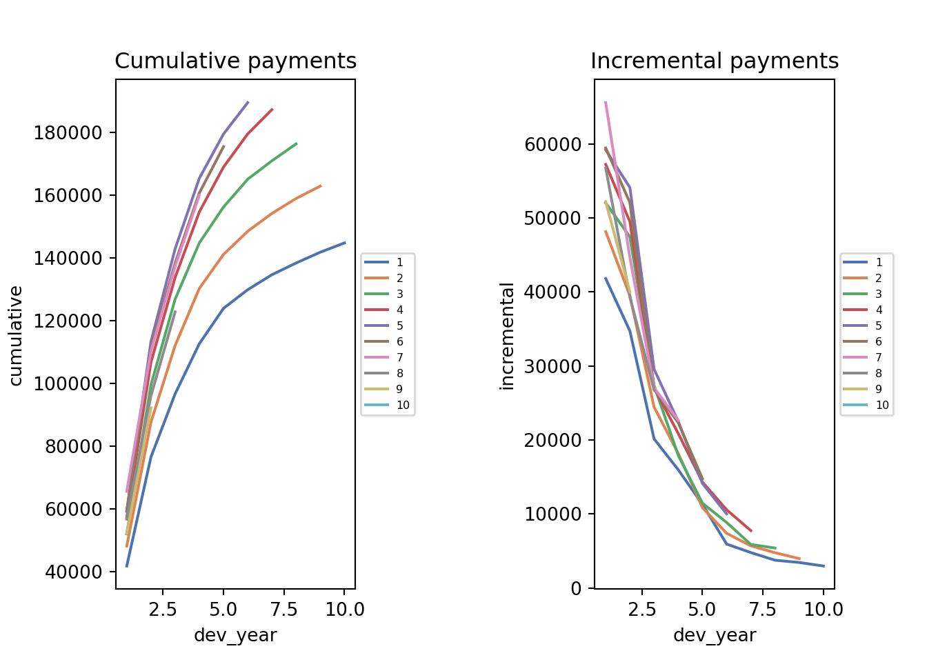
The data look quite well behaved - each year seems to have a similar development pattern.
Before we go further, we’ll add some additional variables to the data set:
- Categorical (or factor) versions of ‘acc_year’ and ‘dev_year’ - these will be needed later for modelling
- A calendar year variable, ‘cal_year’
Later on we’ll need to be able to apply the same categorical structure to subsets of ‘acc_year’ and ‘dev_year’ so we make an object to hold the categorisation, ‘cat_type’.
We’ll have a look at the data and check the variable types to ensure everything is as it should be.
cat_type = pd.api.types.CategoricalDtype(categories=list(range(1,11)), ordered=True)

msdata["acc_year_factor"] = msdata["acc_year"].astype(cat_type)
msdata["dev_year_factor"] = msdata["dev_year"].astype(cat_type)
msdata["cal_year"] = msdata["acc_year"] + msdata["dev_year"] - 1  # subtract 1 so that first cal_year is 1 not 2

print(msdata.head(6))
acc_year dev_year cumulative ... acc_year_factor dev_year_factor cal_year
0 1 1 41821.0 ... 1 1 1
1 1 2 76550.0 ... 1 2 2
2 1 3 96697.0 ... 1 3 3
3 1 4 112662.0 ... 1 4 4
4 1 5 123947.0 ... 1 5 5
5 1 6 129871.0 ... 1 6 6
[6 rows x 7 columns]print(msdata.dtypes)acc_year int32
dev_year int32
cumulative float64
incremental float64
acc_year_factor category
dev_year_factor category
cal_year int32
dtype: objectChain ladder model
Fitting the model
Our first model will be the familiar chain ladder (volume all) model. The monograph (and references therein) note that certain types of GLM gives exactly the same result as the chain ladder so I’m going to use that to get the chain ladder result.
The specific model I’m using that replicates the chain ladder result is the Over-dispersed Poisson (ODP) cross classified (cc) model (Sections 3.3.2 and 3.3.3 of the monograph).
To apply the model, we will use the glm() function from the statsmodels.formula.api package. The cross-classified model requires separate levels for each of accident and development year so we use the categorical versions of these variates.
To fit an ODP model, we use the scale='X2' argument to fit() - the X2 stands for chi-squared and tells glm() to use a Pearson chi-squared estimate for the scale parameter.
The -1 in the model formula instructs glm() to fit without an intercept. Doing this will allow us to recover parameter estimates similar to those in the monograph.
glm_fit1 = smf.glm('incremental~ -1 + acc_year_factor + dev_year_factor',
                   data = msdata,
                   family = sm.families.Poisson() ).fit(scale='X2')
print(glm_fit1.summary())
Generalized Linear Model Regression Results
==============================================================================
Dep. Variable: incremental No. Observations: 55
Model: GLM Df Residuals: 36
Model Family: Poisson Df Model: 18
Link Function: Log Scale: 114.54
Method: IRLS Log-Likelihood: -20.828
Date: Sun, 13 Nov 2022 Deviance: 4128.1
Time: 13:43:06 Pearson chi2: 4.12e+03
No. Iterations: 7 Pseudo R-squ. (CS): 1.000
Covariance Type: nonrobust
=========================================================================================
coef std err z P>|z| [0.025 0.975]
-----------------------------------------------------------------------------------------
acc_year_factor[1] 10.6568 0.032 336.795 0.000 10.595 10.719
acc_year_factor[2] 10.7953 0.030 360.507 0.000 10.737 10.854
acc_year_factor[3] 10.8992 0.029 377.465 0.000 10.843 10.956
acc_year_factor[4] 10.9890 0.028 391.327 0.000 10.934 11.044
acc_year_factor[5] 11.0388 0.028 396.654 0.000 10.984 11.093
acc_year_factor[6] 11.0159 0.029 385.868 0.000 10.960 11.072
acc_year_factor[7] 11.0081 0.029 373.734 0.000 10.950 11.066
acc_year_factor[8] 10.8905 0.033 333.463 0.000 10.826 10.955
acc_year_factor[9] 10.8361 0.037 295.349 0.000 10.764 10.908
acc_year_factor[10] 10.6911 0.051 209.454 0.000 10.591 10.791
dev_year_factor[T.2] -0.2047 0.023 -8.993 0.000 -0.249 -0.160
dev_year_factor[T.3] -0.7474 0.028 -26.512 0.000 -0.803 -0.692
dev_year_factor[T.4] -1.0167 0.033 -30.954 0.000 -1.081 -0.952
dev_year_factor[T.5] -1.4516 0.042 -34.446 0.000 -1.534 -1.369
dev_year_factor[T.6] -1.8325 0.055 -33.495 0.000 -1.940 -1.725
dev_year_factor[T.7] -2.1403 0.072 -29.933 0.000 -2.280 -2.000
dev_year_factor[T.8] -2.3483 0.093 -25.218 0.000 -2.531 -2.166
dev_year_factor[T.9] -2.5132 0.127 -19.831 0.000 -2.762 -2.265
dev_year_factor[T.10] -2.6645 0.199 -13.369 0.000 -3.055 -2.274
=========================================================================================Loss reserve
Now we’ll have a look at the loss reserve. If you’ve done the chain ladder calculations, you should find this gives the same answer.
Before we get there, we’ll write a function to produce a data set from a vectors of acc_year and dev_year variables - this will be useful later on as well.
The function below takes in numpy 1-d arrays of acc and dev and the categorisation we created above and produces a pandas dataframe with the various covariates that we have created so far.
# Write a function to create part of a triangle

def CreateData(acc, dev, cat_type):
    '''
    Creates a data set to apply predict function to

    Parameters
    -------------------------
    acc: np 1-d array of acc values
    dev: np 1-d array of dev values
    It is possible for one of these to be length 1 and this gets repeated

    Returns
    -------------------------
    df with all the various terms that we need:
      acc_year
      dev_year
      acc_year_factor
      dev_year_factor
      cal_year

    '''

    if acc.size == dev.size:
        df = pd.DataFrame({'acc_year': acc, 'dev_year': dev})
    elif acc.size == 1:
        df = pd.DataFrame({'acc_year': np.repeat(acc, dev.size), 'dev_year': dev})
    elif dev.size == 1:
        df = pd.DataFrame({'acc_year': acc, 'dev_year': np.repeat(dev, acc.size)})
    else:
        print("Length of acc and dev must be equal or one must contain one element only")
        return

    # add the other variables and fix types
    df['cal_year'] = df['acc_year'] + df['dev_year'] - 1
    df['acc_year_factor'] = df['acc_year'].astype(cat_type)
    df['dev_year_factor'] = df['dev_year'].astype(cat_type)

    df= df.astype(dtype={'acc_year': int,
                         'dev_year': int,
                         'cal_year': int
                                   })

    return df
We now use this function and give it:
- An accident array that repeats the numbers 1-10 10 times each
- A development array that repeats the sequence 1-10 10 times
- Our previously defined
cat_type
This outputs the full reserving data set (upper and lower triangles) in long form.
We then subset this to keep only the future (lower triangle) data and reindex (number the rows). Finally we create a column that holds the fitted values from our first model.
fulltr = CreateData(acc = np.repeat(np.arange(1,11), 10),
                    dev = np.tile(np.arange(1,11), 10),
                    cat_type = cat_type)

# extract lower tri - make a deep copy so it exists independently of
# fulltr rather than being a slice

futdata = fulltr[fulltr['cal_year']>10].copy(deep=True)

# reindex this
futdata.index = np.arange(0, 45, dtype=int)


futdata['fitted1'] = glm_fit1.predict(futdata)

print(futdata.head())
acc_year dev_year cal_year acc_year_factor dev_year_factor fitted1
0 2 10 11 2 10 3397.665217
1 3 9 11 3 9 4385.341383
2 3 10 12 3 10 3769.510642
3 4 8 11 4 8 5657.645836
4 4 9 12 4 9 4797.591370Now we can look at the OCL by accident year and in total.
# now get ocl by accident year
ocl_year = futdata.groupby(by="acc_year").sum()
print(ocl_year['fitted1'])
acc_year
2 3397.665217
3 8154.852025
4 14579.105829
5 22645.065096
6 31865.349506
7 45753.129496
8 60093.456331
9 80983.200079
10 105874.473778
Name: fitted1, dtype: float64
ocl_total = ocl_year['fitted1'].sum()
print(ocl_total)373346.29735591734Model diagnostics
Calculations
So far, we’ve fitted a model and have calculated the loss reserve. We can do all this with the chain ladder algorithm. Now we start looking at some of the extras that using a GLM gives us - for a start the statistical model structure means that we can calculate residuals with known properties, assuming the assumptions underlying the model are valid.
If the model assumptions are satisfied by the data, then the residuals should not have any remaining structure. Plots of residuals can therefore be useful to detect violations of model assumptions. Note that we need to be careful to use the right types of residuals - in many cases we want to use standardised deviance residuals:
- Deviance residuals because the more recognisable Pearson residuals (based on actual - fitted) are difficult to interpret for non-normal models.
- Standardised because the raw residuals are on different scales depending on the scale of the underlying values.
Some more details may be found in Chapter 6 of the monograph and also in Chapter 5 of A Practitioner’s Introduction to Stochastic Reserving.
Here we look at the following:
- Residual Scatterplots
- by linear predictor
- by accident, development and calendar years
- if the model assumptions are satisfied then the residuals should look homogeneous (or in layperson’s language, like a random cloud), centred around zero)
- Heat map of actual vs fitted laid out in triangular form
- In this we get the actual/fitted ratio in each (acc, dev) cell (subject to lower and upper bounds of [0.5, 2]) and then plot the colour-coded triangle of the actual/fitted values
- heat maps are helpful to check for model fit and may help to identify missing interactions.
We have to prepare the data by adding the fitted values and residuals.
Because this model has a lot of parameters, there are two observations where the fitted is exactly equal to the actual – (acc_year=1, dev_year=10) and (acc_year=10, dev_year=1). This is because these observations have a unique parameter.
statsmodels returns unstandardised deviance residuals, so we’ve included a function to calculate the standardised versions.
The deviance calculations below return
nan(not a number) andinffor these points, but the residual should really be 0 so this adjustment is made manually.Also add actual/fitted ratios and the log of these (restricted to the range [log(0.5), log(2)]) - these will be used for a heatmap later.
- The restricted range is used to generate easier to read shadings in the heat-map, while the conversion to log means that the shading scales will be similar intensity for \(x\)% and \(1/x\) %
First, here’s a function to calculate standardised deviance residuals.
# Write a function to calculate std deviance residuals
# statsmodels just gives deviance residuals, but we want standardised.
# For definitions of these residuals consult (e.g) http://documentation.sas.com/doc/en/pgmsascdc/9.4_3.4/statug/statug_genmod_details25.htm
#
# to calculate standardised deviance residuals:
#  - resid_deviance from statsmodels = sqrt(di) sign(y-mu)
#  - std_resid_deviance = sqrt(di) sign(y-mu) / sqrt(phi (1-hat matrix))

def StdDevResids(df, glm_obj, resid_colname = 'std_dev_resid'):
    '''
    Calculates the standardised deviance residuals.

    Parameters
    -------------------------
    df: Pandas dataframe to which we add the residuals - should have dimensions of training/model data
    glm_obj: Statsmodel glm object containing results of fit
    resid_colname = name of residual column name

    Returns
    -------------------------
    df updated with std resids column, called resid_colname

    resid_deviance = sqrt(di) sign(y-mu) - stored in glm_obj
    std_resid_deviance = sqrt(di) sign(y-mu) / sqrt(phi (1-hat matrix)) - calculated
    For definitions of these residuals consult http://documentation.sas.com/doc/en/pgmsascdc/9.4_3.4/statug/statug_genmod_details25.htm


    '''

    # calculate residuals
    df[resid_colname] = glm_obj.resid_deviance / (np.sqrt(glm_obj.scale * (1 - glm_obj.get_hat_matrix_diag())))

    # when actual=fitted can get nans and infs in results so replace these with zero
    df[resid_colname].replace(np.nan,0, inplace = True)
    df[resid_colname].replace(np.inf,0, inplace = True)

    return(df)
Now calculate the residuals, and add fitted values and the AvsF values as well.
There will be a warning message from the residual calculation function - this relates to the cells where actual == fitted and can be ignored.
msdata = StdDevResids(msdata, glm_fit1, 'residuals1')<string>:23: RuntimeWarning: invalid value encountered in sqrtmsdata['fitted1'] = glm_fit1.predict(msdata)
msdata['linear_predictor1'] = glm_fit1.predict(msdata, linear=True)
msdata['AvsF1'] = msdata['incremental'] / msdata['fitted1']
msdata['AvsF_restricted1'] = np.log(np.maximum(0.5, np.minimum(2, msdata['AvsF1'])))
msdata.head(10) acc_year dev_year ... AvsF1 AvsF_restricted1
0 1 1 ... 0.984516 -1.560475e-02
1 1 2 ... 1.003241 3.235741e-03
2 1 3 ... 1.001466 1.464611e-03
3 1 4 ... 1.038796 3.806213e-02
4 1 5 ... 1.134358 1.260672e-01
5 1 6 ... 0.871577 -1.374512e-01
6 1 7 ... 0.955659 -4.535425e-02
7 1 8 ... 0.922093 -8.110930e-02
8 1 9 ... 0.998183 -1.818724e-03
9 1 10 ... 1.000000 7.771561e-15
[10 rows x 12 columns]Plotting
Now let’s look at the residual scatterplots. In the linear predictor scatterplot, the points are colour coded by development year.
fig, axs = plt.subplots(2, 2)
plt.subplots_adjust(wspace=1, hspace=1)
g=sns.scatterplot(x='linear_predictor1', y='residuals1',hue=msdata.dev_year, data=msdata, palette=sns.color_palette("deep"), ax=axs[0,1])
g.set_title("Linear Predictor")
g.legend(loc='center left', bbox_to_anchor=(1, 0.5),fontsize = 6)
sns.scatterplot(x='acc_year', y='residuals1', data=msdata,palette=sns.color_palette("deep"), ax=axs[0,0]).set_title("Accident Year")
sns.scatterplot(x='dev_year', y='residuals1', data=msdata,palette=sns.color_palette("deep"), ax=axs[1,0]).set_title("Development Year")
sns.scatterplot(x='cal_year', y='residuals1', data=msdata,palette=sns.color_palette("deep"), ax=axs[1,1]).set_title("Calendar Year")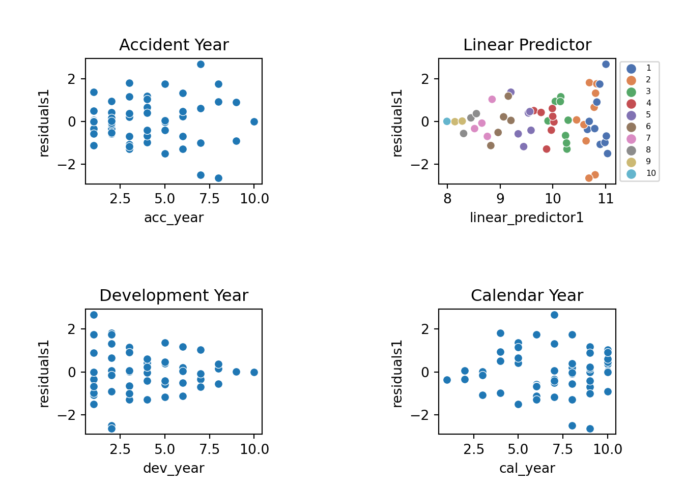
These results are quite good - bear in mind there are only a small number of points so plots must be interpreted in relation to this. In particular:
- The residuals do not appear to fan out or fan in (once you take into account that later development years have small number of points)
- They appear centred around 0
Now construct and draw the heat map. Note that the colours are:
- blue (A/F = 50%)
- white (A/F = 100%)
- red (A/F = 200%)
with shading for in-between values
fig, axs = plt.subplots(1)

cmap = sns.diverging_palette(255,0,sep=16, as_cmap=True)

sns.heatmap(data = msdata.pivot('acc_year','dev_year','AvsF_restricted1'),
            linewidths = .5,
            cmap = cmap,
            center=0,
            cbar = False)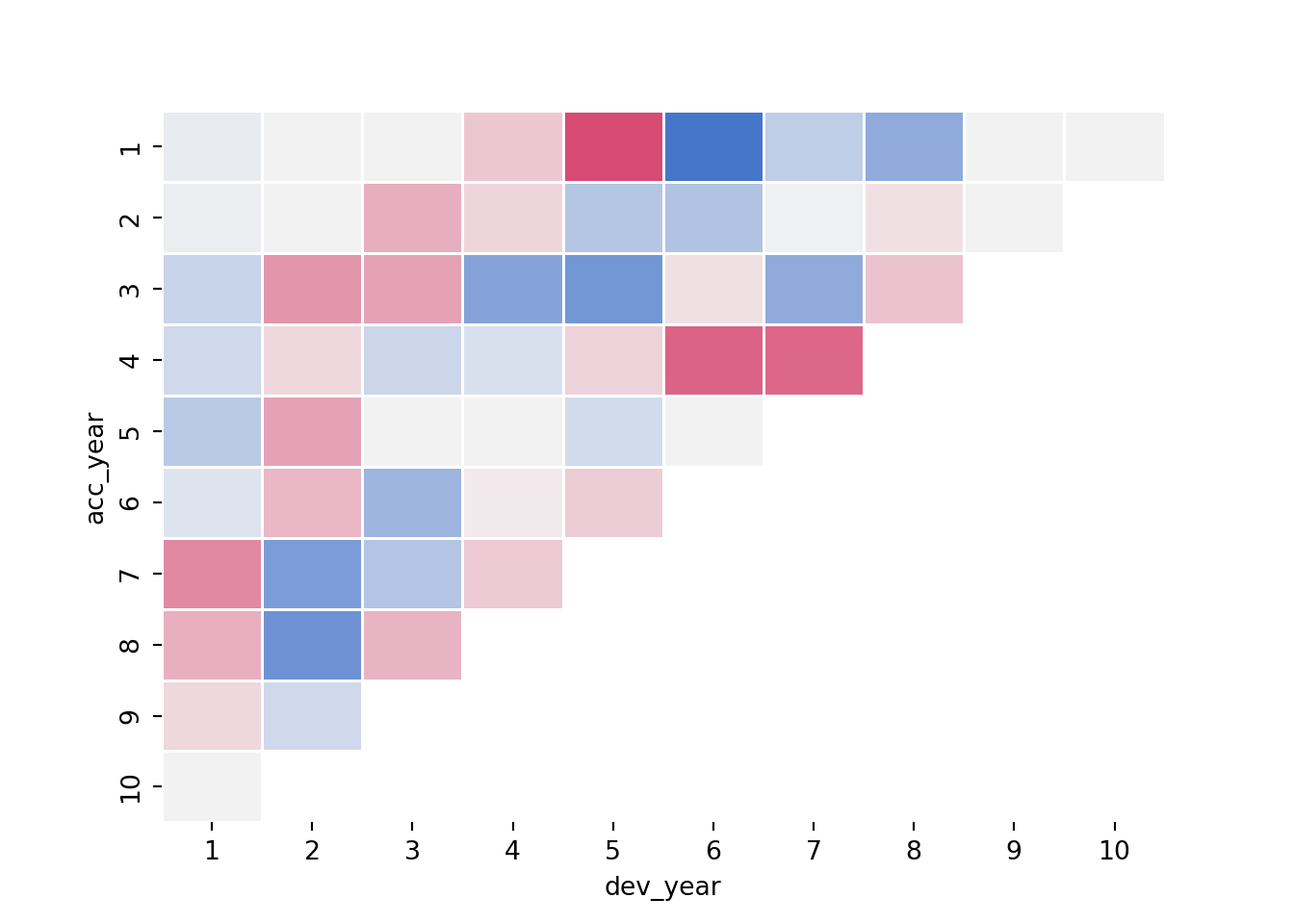
In a heat map for a reserving triangle, we look for a random scattering of red and blue points. This plot looks quite good (though we’ll revisit this shortly).
Refining the model
We could stop here - and just use the results from this model, which match those produced by the chain ladder. The diagnostics suggest that the model fits quite well. However, because this is a GLM, we have more options than just replicating the chain ladder.
In particular, can we:
- identify simplifications to the model to make it more parsimonious (i.e. reduce the number of parameters)?
- identify any areas of poorer fit that may suggest missing model terms including interactions?
Simplifying the model
First we consider if we can use a parametric shape for the accident and development year parameters. The end result should be something similar to the chain ladder approach but with far fewer parameters.
Accident year
First plot the accident year parameters. We could access the parameters directly and plot these, but an alternative way of doing this is to make a data set where we have all values of acc_year and a single value of dev_year - the base level which is a parameter estimate of 0 - and then get the linear predicted values for this. This latter method will be useful later when we refine the model so we’ll use it here too.
We therefore use the CreateData() function we wrote earlier to make a data set in suitable form and then add the linear predicted values to this.
acc_fit = CreateData(acc = np.arange(1,11), dev=np.array(1), cat_type = cat_type)
acc_fit['fitted1'] = glm_fit1.predict(acc_fit, linear = True)

print(acc_fit)
acc_year dev_year cal_year acc_year_factor dev_year_factor fitted1
0 1 1 1 1 1 10.656759
1 2 1 2 2 1 10.795334
2 3 1 3 3 1 10.899190
3 4 1 4 4 1 10.989037
4 5 1 5 5 1 11.038835
5 6 1 6 6 1 11.015898
6 7 1 7 7 1 11.008077
7 8 1 8 8 1 10.890500
8 9 1 9 9 1 10.836129
9 10 1 10 10 1 10.691081
sns.lineplot(x = 'acc_year', y = 'fitted1', marker = 'o', data=acc_fit)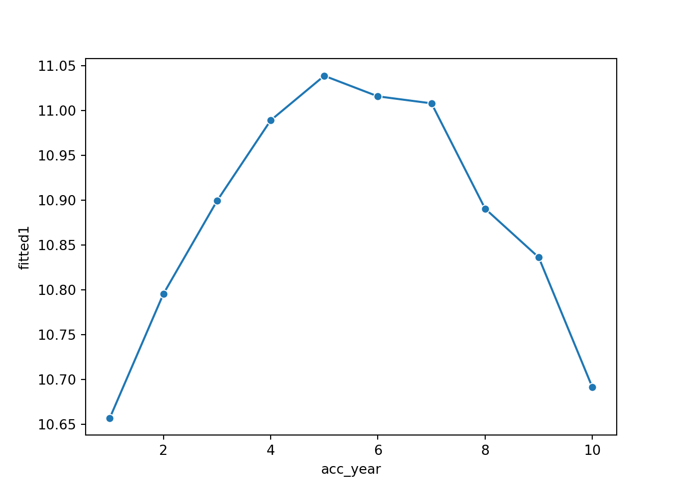
Note that the shape of the accident parameters closely resembles that of a parabola.
This suggests that we can replace the 10 accident year parameters by
- the overall intercept
- an
acc_yearterm - an
acc_yearsquared term (we’ll need to add this to the dataframe)
So refit the model on this basis:
- Drop the -1 from the
glm_fit1formula to allow the model to have an intercept - Replace the
acc_year_factorterm with the parabola terms.
msdata["acc_year_2"] = np.power(msdata["acc_year"], 2)

glm_fit2 = smf.glm('incremental ~ acc_year + acc_year_2 + dev_year_factor',
                   data = msdata,
                   family = sm.families.Poisson() ).fit(scale='X2')
print(glm_fit2.summary())
Generalized Linear Model Regression Results
==============================================================================
Dep. Variable: incremental No. Observations: 55
Model: GLM Df Residuals: 43
Model Family: Poisson Df Model: 11
Link Function: Log Scale: 102.58
Method: IRLS Log-Likelihood: -24.714
Date: Sun, 13 Nov 2022 Deviance: 4427.0
Time: 13:43:49 Pearson chi2: 4.41e+03
No. Iterations: 7 Pseudo R-squ. (CS): 1.000
Covariance Type: nonrobust
=========================================================================================
coef std err z P>|z| [0.025 0.975]
-----------------------------------------------------------------------------------------
Intercept 10.4710 0.034 304.264 0.000 10.404 10.538
dev_year_factor[T.2] -0.2056 0.021 -9.661 0.000 -0.247 -0.164
dev_year_factor[T.3] -0.7501 0.026 -28.314 0.000 -0.802 -0.698
dev_year_factor[T.4] -1.0148 0.031 -32.755 0.000 -1.076 -0.954
dev_year_factor[T.5] -1.4520 0.040 -36.484 0.000 -1.530 -1.374
dev_year_factor[T.6] -1.8305 0.052 -35.432 0.000 -1.932 -1.729
dev_year_factor[T.7] -2.1422 0.068 -31.734 0.000 -2.274 -2.010
dev_year_factor[T.8] -2.3527 0.088 -26.758 0.000 -2.525 -2.180
dev_year_factor[T.9] -2.5137 0.120 -21.011 0.000 -2.748 -2.279
dev_year_factor[T.10] -2.6609 0.188 -14.167 0.000 -3.029 -2.293
acc_year 0.2001 0.014 14.071 0.000 0.172 0.228
acc_year_2 -0.0179 0.001 -13.210 0.000 -0.021 -0.015
=========================================================================================Now let’s compare the previous and current fit. We go back to the acc_fit dataframe and add the linear predicted values from the glm_fit2 model (and hopefully it now becomes clearer why it can be convenient to use a data set with the predict() method rather than accessing parameter estimates directly.
# Plot the values before and after

# first add acc_year_2 to acc_fit
acc_fit["acc_year_2"] = np.power(acc_fit["acc_year"], 2)

# add glm_fit2 linpred
acc_fit['fitted2'] = glm_fit2.predict(acc_fit, linear = True)

print(acc_fit)
acc_year dev_year cal_year ... fitted1 acc_year_2 fitted2
0 1 1 1 ... 10.656759 1 10.653146
1 2 1 2 ... 10.795334 4 10.799501
2 3 1 3 ... 10.899190 9 10.910041
3 4 1 4 ... 10.989037 16 10.984768
4 5 1 5 ... 11.038835 25 11.023682
5 6 1 6 ... 11.015898 36 11.026781
6 7 1 7 ... 11.008077 49 10.994067
7 8 1 8 ... 10.890500 64 10.925539
8 9 1 9 ... 10.836129 81 10.821197
9 10 1 10 ... 10.691081 100 10.681042
[10 rows x 8 columns]
sns.lineplot(x = 'acc_year',
             y = 'value',
             hue = 'variable',
             marker = 'o',
             data=pd.melt(acc_fit[['acc_year', 'fitted1', 'fitted2']], 'acc_year'))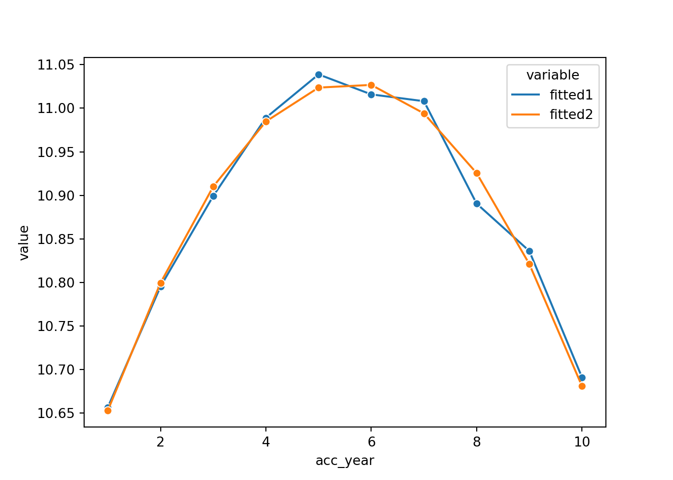
This looks very good - the fit is very similar, but we have 7 fewer parameters.
Development year
Now we do the same thing for development year - we build a dataset with all dev_year levels and acc_year set the the same value (I’ve chosen 1) and then we calculate the linear predicted values and plot these.
dev_fit = CreateData(acc = np.array(1), dev=np.arange(1,11), cat_type = cat_type)
dev_fit["acc_year_2"] = np.power(dev_fit["acc_year"] ,2)
dev_fit['fitted2'] = glm_fit2.predict(dev_fit, linear = True)

sns.lineplot(x = 'dev_year', y = 'fitted2', marker = 'o', data=dev_fit)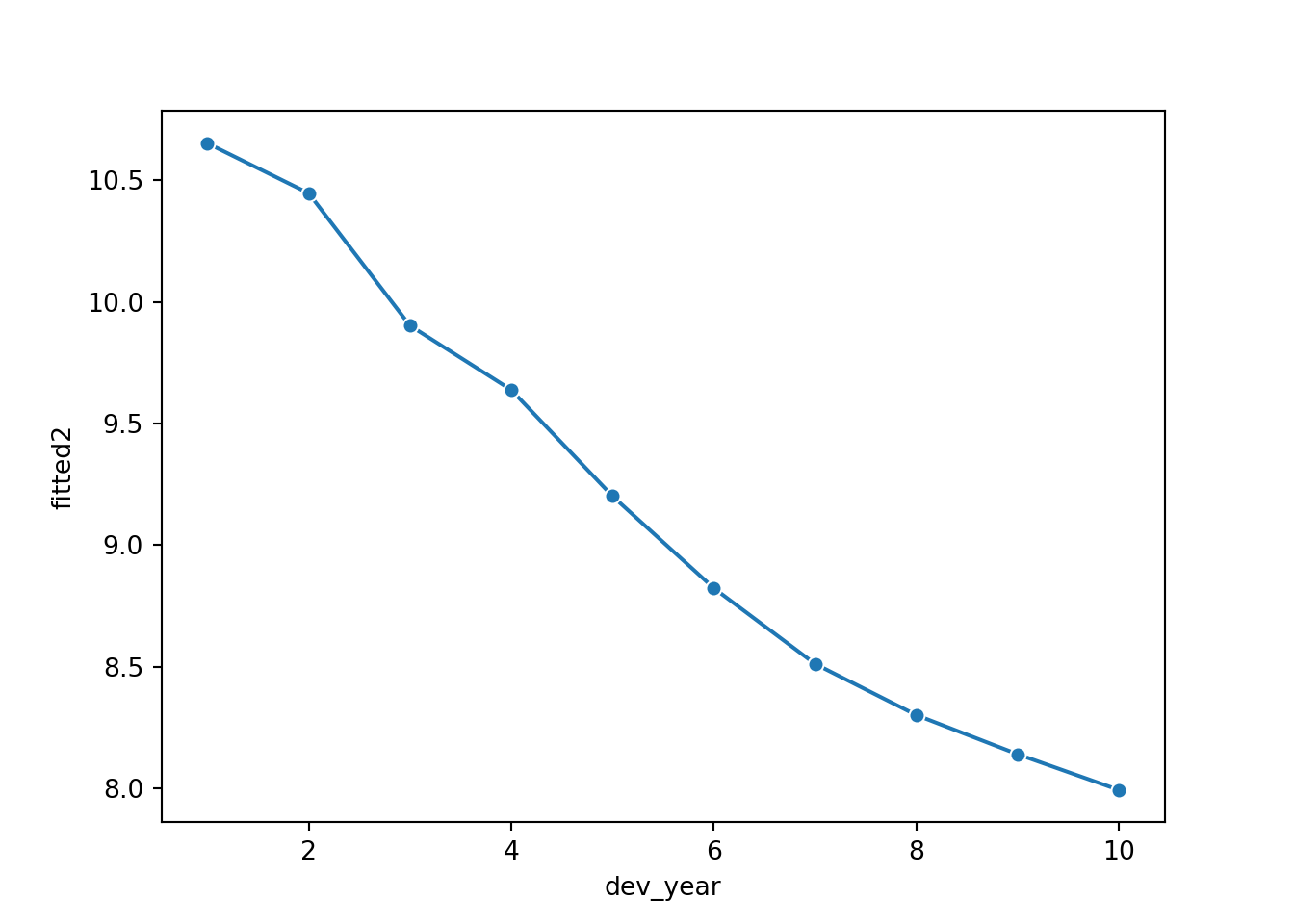
Looking at this plot, it appears that a straight line would fit quite well. However, this fit would be improved by allowing the straight line to bend (have a knot) at dev_year = 7. So let’s try this below.
Note we actually fit dev_year - 1 rather than dev_year. This means that the parameter estimate at dev_year = 1 is 0, just as it is in the glm_fit2 model.
msdata['dev_year_m1'] = msdata["dev_year"] - 1
msdata['dev_year_ge_7'] = np.maximum(msdata["dev_year"] - 7.5, 0)

glm_fit3 = smf.glm('incremental ~ acc_year + acc_year_2 + dev_year_m1 + dev_year_ge_7',
                   data = msdata,
                   family = sm.families.Poisson() ).fit(scale='X2')
print(glm_fit3.summary())
Generalized Linear Model Regression Results
==============================================================================
Dep. Variable: incremental No. Observations: 55
Model: GLM Df Residuals: 50
Model Family: Poisson Df Model: 4
Link Function: Log Scale: 242.06
Method: IRLS Log-Likelihood: -25.865
Date: Sun, 13 Nov 2022 Deviance: 11879.
Time: 13:44:08 Pearson chi2: 1.21e+04
No. Iterations: 7 Pseudo R-squ. (CS): 1.000
Covariance Type: nonrobust
=================================================================================
coef std err z P>|z| [0.025 0.975]
---------------------------------------------------------------------------------
Intercept 10.5095 0.052 201.734 0.000 10.407 10.612
acc_year 0.2042 0.022 9.451 0.000 0.162 0.247
acc_year_2 -0.0183 0.002 -8.891 0.000 -0.022 -0.014
dev_year_m1 -0.3641 0.009 -41.160 0.000 -0.381 -0.347
dev_year_ge_7 0.2389 0.088 2.701 0.007 0.066 0.412
=================================================================================Assuming the fit is satisfactory, our original model with 19 parameters has now been simplified to 5 parameters - much more parsimonious and robust.
Let’s check the fit by dev_year to see.
# check fit by dev_year

dev_fit['dev_year_m1'] = dev_fit["dev_year"] - 1
dev_fit['dev_year_ge_7'] = np.maximum(dev_fit["dev_year"] - 7.5, 0)

dev_fit['fitted3'] = glm_fit3.predict(dev_fit, linear = True)

sns.lineplot(x = 'dev_year',
             y = 'value',
             hue = 'variable',
             marker = 'o',
             data=pd.melt(dev_fit[['dev_year', 'fitted2', 'fitted3']], 'dev_year'))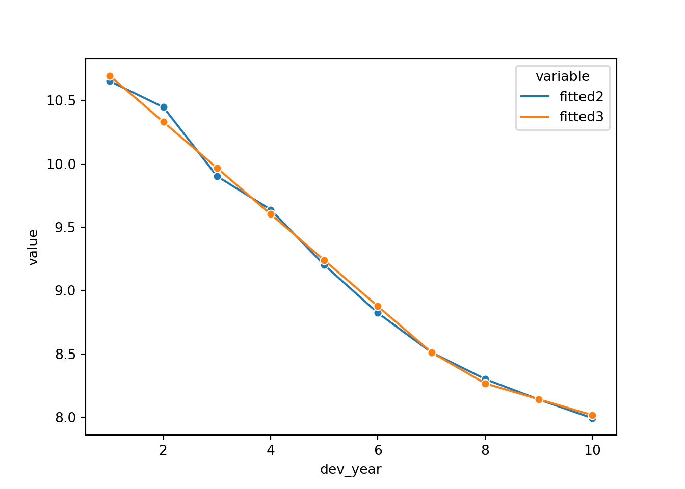
This looks good. However dev_year = 2 is a bit underfit in the latest model, so we can add something to improve this fit (a term at dev_year=2). Refit and replot.
# add dq_eq_2 term

msdata['dev_year_eq_2'] = 1 * (msdata["dev_year"] == 2)

glm_fit4 = smf.glm('incremental ~ acc_year + acc_year_2 + dev_year_m1 + dev_year_ge_7 + dev_year_eq_2',
                   data = msdata,
                   family = sm.families.Poisson() ).fit(scale='X2')
print(glm_fit4.summary())
Generalized Linear Model Regression Results
==============================================================================
Dep. Variable: incremental No. Observations: 55
Model: GLM Df Residuals: 49
Model Family: Poisson Df Model: 5
Link Function: Log Scale: 107.27
Method: IRLS Log-Likelihood: -27.579
Date: Sun, 13 Nov 2022 Deviance: 5273.8
Time: 13:44:17 Pearson chi2: 5.26e+03
No. Iterations: 7 Pseudo R-squ. (CS): 1.000
Covariance Type: nonrobust
=================================================================================
coef std err z P>|z| [0.025 0.975]
---------------------------------------------------------------------------------
Intercept 10.4687 0.035 297.896 0.000 10.400 10.538
acc_year 0.2001 0.014 13.867 0.000 0.172 0.228
acc_year_2 -0.0179 0.001 -13.018 0.000 -0.021 -0.015
dev_year_m1 -0.3577 0.006 -59.405 0.000 -0.370 -0.346
dev_year_ge_7 0.2356 0.059 3.996 0.000 0.120 0.351
dev_year_eq_2 0.1545 0.019 7.932 0.000 0.116 0.193
=================================================================================
# check fit by dev_year

dev_fit['dev_year_eq_2'] = 1 * (dev_fit["dev_year"] == 2)

dev_fit['fitted4'] = glm_fit4.predict(dev_fit, linear = True)

sns.lineplot(x = 'dev_year',
             y = 'value',
             hue = 'variable',
             marker = 'o',
             data=pd.melt(dev_fit[['dev_year', 'fitted2', 'fitted3', 'fitted4']], 'dev_year'))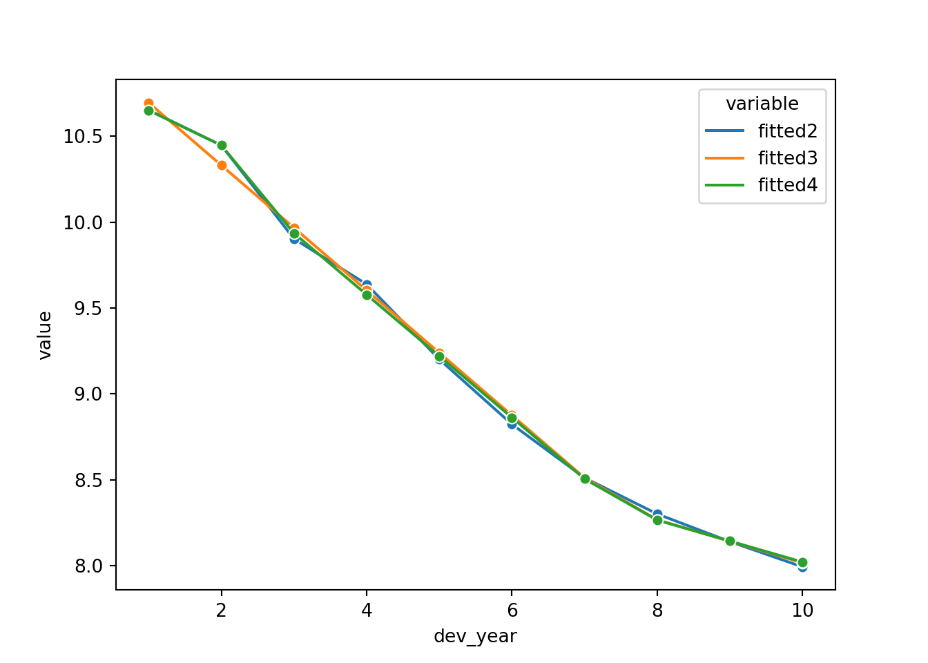
Looks good! Fitting dev_year=2 better has also improved the tail fitting (dev_year>7).
Identifying missing structure
The second part of the model refining process involves checking for missing structure.
Let’s have a better look at the heat map, as it stands after the model simplification process.
# look at heat map again - remember log scale

msdata['fitted4'] = glm_fit4.predict(msdata)
msdata['AvsF4'] = msdata['incremental'] / msdata['fitted4']
msdata['AvsF_restricted4'] = np.log(np.maximum(0.5, np.minimum(2, msdata['AvsF4'])))

fig, axs = plt.subplots(1)

sns.heatmap(data = msdata.pivot('acc_year', 'dev_year', 'AvsF_restricted4'),
            linewidths = .5,
            cmap = cmap,
            center=0,
            cbar=False)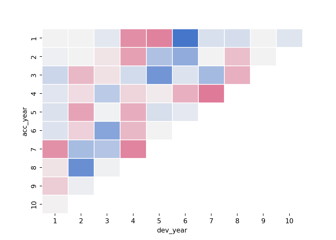
Let’s refer to the annotated version of this plot from the previous version of this article in R. Note that the heatmap colours are a little different, but the underlying values are the same.
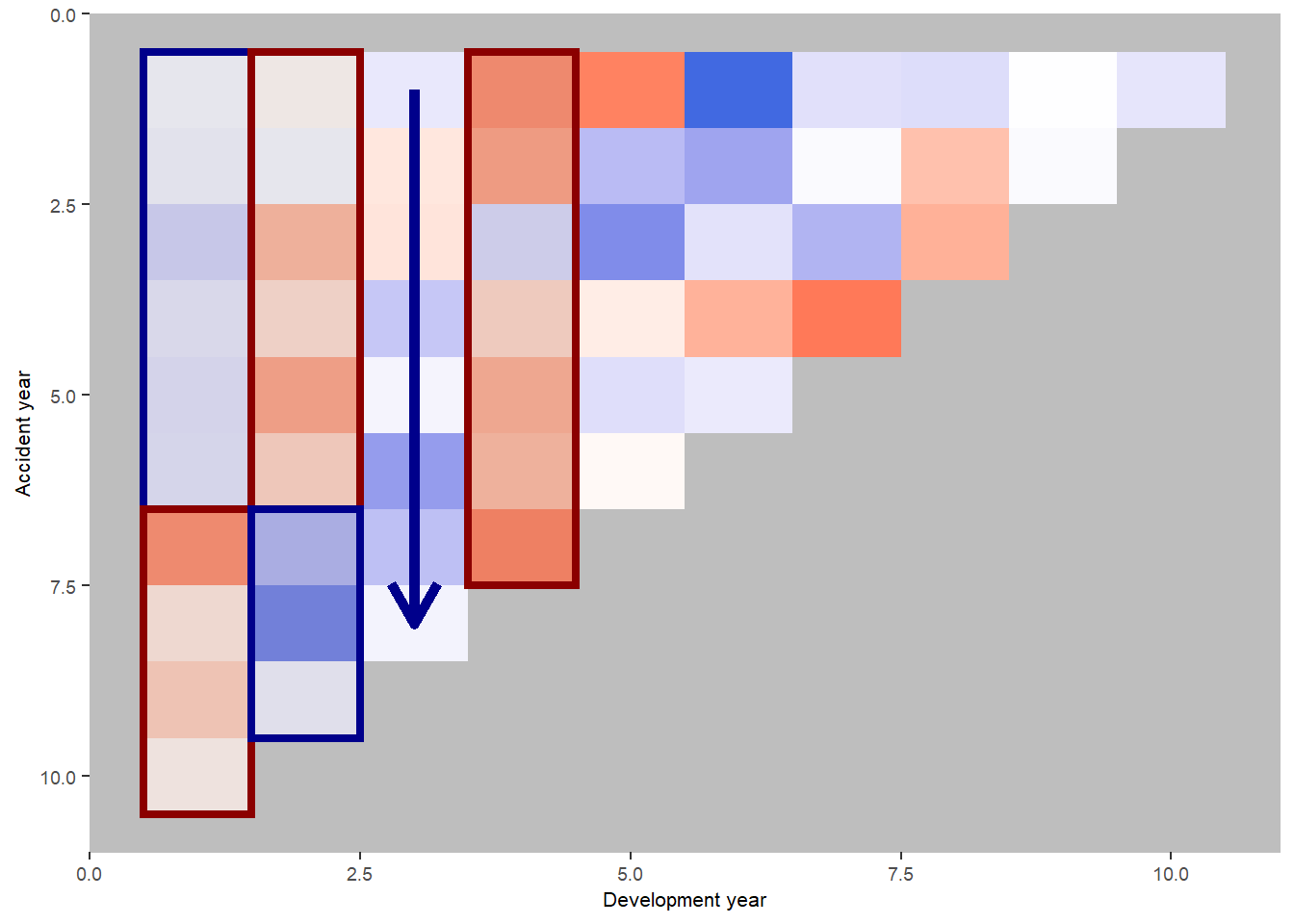
We see:
- development year 1, a distinct area of blue in the earlier accident years (A < F), followed by red (A > F)
- development year 2, a distinct area of red in the earlier accident years (A > F), followed by blue (A < F)
- development year 3, a possible progression from red to blue with increasing accident year (F increasing relative to A)
- development year 4, nearly all red (A > F)
This suggests the payment pattern has altered and can be accommodated by (mostly) interaction terms within the GLM. Consider adding the following terms:
- (development year = 1) * (accident year is between 1 and 6)
- (development year = 2) * (accident year is between 1 and 6)
- (development year = 3) * (accident year linear trend)
- (development year = 4)
So, let’s refit the model with terms to capture these and have a look at the heat map again
# fit model with interactions
msdata['dev_year_eq_1'] = 1 * (msdata["dev_year"] == 1)
msdata['dev_year_eq_3'] = 1 * (msdata["dev_year"] == 3)
msdata['dev_year_eq_4'] = 1 * (msdata["dev_year"] == 4)
msdata['acc_year_1_6']  = 1 * (msdata['acc_year'] >= 1)*(msdata['acc_year'] <= 6)

formula4 = 'incremental ~ acc_year + acc_year_2 + dev_year_m1 + dev_year_ge_7 + dev_year_eq_2'  # previous model
formula5 = formula4 + ' + dev_year_eq_4 + dev_year_eq_1:acc_year_1_6 +  dev_year_eq_2:acc_year_1_6 + dev_year_eq_3:acc_year'


glm_fit5 = smf.glm(formula5,
                   data = msdata,
                   family = sm.families.Poisson() ).fit(scale='X2')
print(glm_fit5.summary())
Generalized Linear Model Regression Results
==============================================================================
Dep. Variable: incremental No. Observations: 55
Model: GLM Df Residuals: 45
Model Family: Poisson Df Model: 9
Link Function: Log Scale: 53.933
Method: IRLS Log-Likelihood: -28.461
Date: Sun, 13 Nov 2022 Deviance: 2426.9
Time: 13:44:29 Pearson chi2: 2.43e+03
No. Iterations: 7 Pseudo R-squ. (CS): 1.000
Covariance Type: nonrobust
==============================================================================================
coef std err z P>|z| [0.025 0.975]
----------------------------------------------------------------------------------------------
Intercept 10.4904 0.032 327.787 0.000 10.428 10.553
acc_year 0.2066 0.011 19.007 0.000 0.185 0.228
acc_year_2 -0.0183 0.001 -16.078 0.000 -0.021 -0.016
dev_year_m1 -0.3685 0.007 -53.317 0.000 -0.382 -0.355
dev_year_ge_7 0.2720 0.044 6.145 0.000 0.185 0.359
dev_year_eq_2 0.0375 0.025 1.518 0.129 -0.011 0.086
dev_year_eq_4 0.0528 0.024 2.217 0.027 0.006 0.099
dev_year_eq_1:acc_year_1_6 -0.0671 0.028 -2.392 0.017 -0.122 -0.012
dev_year_eq_2:acc_year_1_6 0.1273 0.031 4.101 0.000 0.066 0.188
dev_year_eq_3:acc_year -0.0113 0.004 -2.913 0.004 -0.019 -0.004
==============================================================================================This model should match that displayed in Table 7-5 of the monograph - and indeed it does (some very minor differences in parameter values - the model in the monograph was fitted in SAS).
Look at the updated heat map again - has the model resolved the identified issues?
msdata['fitted5'] = glm_fit5.predict(msdata)
msdata['AvsF5'] = msdata['incremental'] / msdata['fitted5']
msdata['AvsF_restricted5'] = np.log(np.maximum(0.5, np.minimum(2, msdata['AvsF5'])))


fig, axs = plt.subplots(1)


sns.heatmap(data = msdata.pivot('acc_year', 'dev_year', 'AvsF_restricted5'),
            linewidths = .5,
            cmap = cmap,
            center=0,
            cbar=False)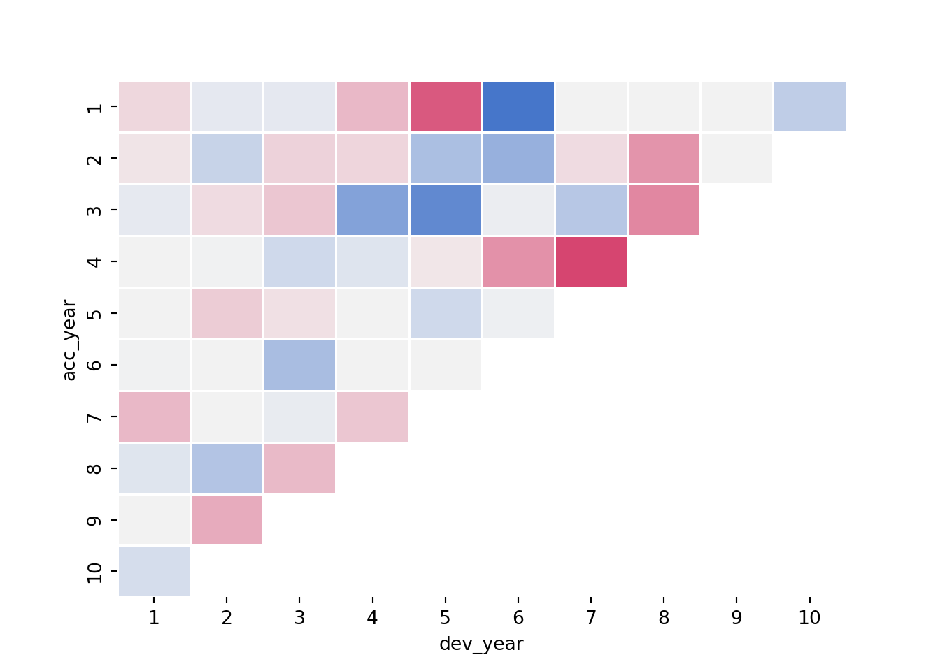
Here’s the annotated R plot which helps show the impact of the interactions

This looks much better.
We should also look at the residual plots again
# look at residual plots again

msdata = StdDevResids(msdata, glm_fit5, 'residuals5')
msdata['linear_predictor5'] = glm_fit5.predict(msdata, linear = True)

fig, axs = plt.subplots(2, 2)
plt.subplots_adjust(wspace=1, hspace=1)
g=sns.scatterplot(x='linear_predictor5', y='residuals5',hue=msdata.dev_year, data=msdata, palette=sns.color_palette("deep"), ax=axs[0,1])
g.set_title("Linear Predictor")
g.legend(loc='center left', bbox_to_anchor=(1, 0.5),fontsize = 6)
sns.scatterplot(x='acc_year', y='residuals5', data=msdata,palette=sns.color_palette("deep"), ax=axs[0,0]).set_title("Accident Year")
sns.scatterplot(x='dev_year', y='residuals5', data=msdata,palette=sns.color_palette("deep"), ax=axs[1,0]).set_title("Development Year")
sns.scatterplot(x='cal_year', y='residuals5', data=msdata,palette=sns.color_palette("deep"), ax=axs[1,1]).set_title("Calendar Year")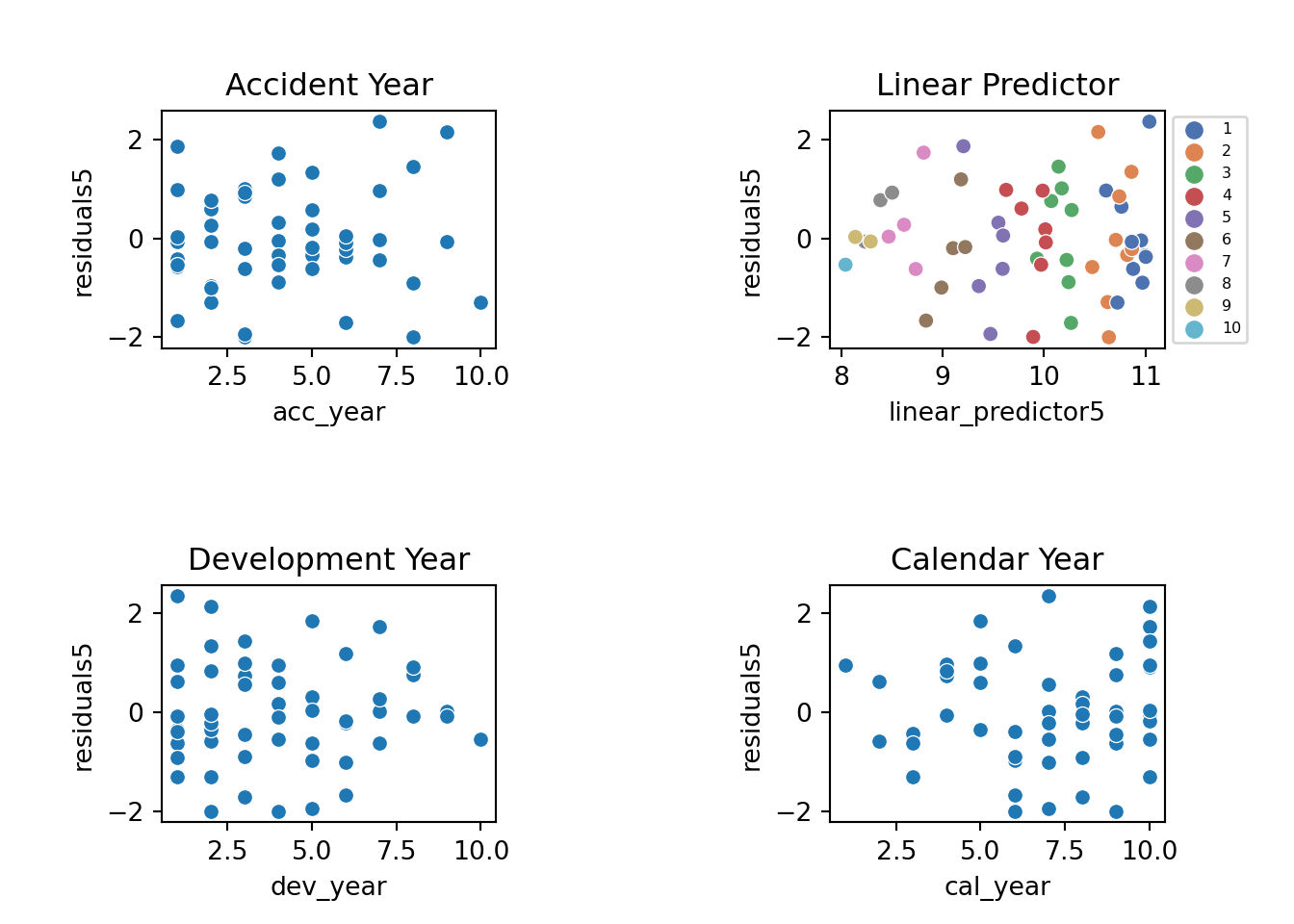
These residuals do look better than those from the chain ladder model.
Loss reserve
Now that we have a model, let’s produce the estimate of the outstanding claims by accident year and in total.
- Take the lower triangle data [futdata] created above
- Add on the new variates we created
- Score the model on this data
- Summarise the results
# add all the new terms to futdata
futdata['acc_year_2'] = np.power(futdata['acc_year'], 2)
futdata['dev_year_m1'] = futdata["dev_year"] - 1
futdata['dev_year_ge_7'] = np.maximum(futdata['dev_year'] - 7.5, 0)
futdata['dev_year_eq_2'] = 1*(futdata['dev_year'] == 2)
futdata['dev_year_eq_1'] = 1*(futdata['dev_year'] == 1)
futdata['dev_year_eq_3'] = 1*(futdata['dev_year'] == 3)
futdata['dev_year_eq_4'] = 1*(futdata['dev_year'] == 4)
futdata['acc_year_1_6']  = 1*(futdata['acc_year'] >= 1)*(futdata['acc_year'] <= 6)

futdata['fitted5'] = glm_fit5.predict(futdata)

print(futdata.head(6))
acc_year dev_year cal_year ... dev_year_eq_4 acc_year_1_6 fitted5
0 2 10 11 ... 0 1 3618.769139
1 3 9 11 ... 0 1 4470.907136
2 3 10 12 ... 0 1 4059.634560
3 4 8 11 ... 0 1 5324.840843
4 4 9 12 ... 0 1 4835.016085
5 4 10 13 ... 0 1 4390.249630
[6 rows x 15 columns]Reserves by accident year
ocl_year = futdata.groupby(by='acc_year').sum()
print(ocl_year['fitted5'])
acc_year
2 3618.769139
3 8530.541696
4 14550.106558
5 22172.719479
6 32458.174082
7 45694.907228
8 62955.431279
9 79300.613414
10 101211.917139
Name: fitted5, dtype: float64Total reserves
ocl_total = ocl_year['fitted5'].sum()
print(ocl_total)370493.1800137104Reviewing this example
Looking back over this example, what we have done is started with a chain ladder model and then shown how we can use a GLM to fit a more parsimonious model (i.e. fewer parameters). It may then be possible to reconcile the shape of the parametric fit by accident year to underlying experience in the book - here we saw higher payments in the middle accident years. Is this due to higher claims experience or higher premium volumes? Does this give us an insight that allows us to better extrapolate into the future when setting reserves?
We have also used model diagnostics to identify areas of misfit and then used GLM interactions to capture these changes.
Practical use of GLMs in traditional reserving
Modelling
The ideas in this simple example extend to more complex traditional scenarios. By traditional I mean that the data you have available to you are classified by accident (or underwriting), development and calendar periods only.
First decide what you are going to model. Here we had a single model of incremental payments. However you could fit a Payments Per Claim Finalised (PPCF) model which consists of 3 submodels - numbers of claims incurred by accident period, number of claims finalised by (accident, development period) and payments per claim finalised by (accident, development period). Each of these could then be fitted by a GLM.
For whatever you’re modelling, you then pick the two triangle directions that you think are most critical for that experience. You can’t include all 3 at the start since they are correlated.
So, for PPCF submodels:
- for number of claims incurred models, accident and development period effects are likely to be where you start.
- numbers of claims finalised will usually depend on development period (type of claim) and calendar period (to take account of changes in claim settlement processes)
- for claim size models, you will probably want development and calendar period effects. For these models you could use operational time instead of development period to avoid changes in the timing of claims finalisations impacting your model.
Then fit the models by starting with the modelled effects as factors and use methods such as those outlined above to reduce the number of parameters by using parametric shapes. Look for missing structure and consider adding interactions or (carefully) adding limited functions of the third triangular direction. Take advantage of GLM tools to refine your model. Use what you know about the portfolio to inform your model - if you know that there was a period of rapid claims inflation, then include that in your model.
Setting reserves
It is possible to overlay judgement onto a GLM’s predictions. At the end of the day, the predictions are just based on a mathematical formula. So, taking claims inflation as an example, if you’ve been seeing 5% p.a. over the last 3 years, but you think this is going to moderate going forward, then you can adjust the projections by removing the 5% p.a. rate into the future and replacing it with, say, 2% p.a. Once you get familiar with using GLMs, you might find it easier to incorporate judgement - the GLM can capture more granularity about past experience which in turn may make it easier to work out how things might change in future and how to numerically include these changes.
Additional References
The references below have further examples of fitting GLMs in this way, and show how to capture quite complex experience. Although both use individual data, the methodology can be used in a similar manner for aggregate data.
- Loss Reserving with GLMs: A Case Study
- Individual Claim modelling of CTP data
- Predictive modeling applications in actuarial science, Frees and Derig, 2004 - in particular see Chapter 18 in Volume 1 and Chapter 3 in Volume 2.
Please feel free to add references to other useful material in the comments.