library(SPLICE) # Load the package once installed
library(DT)
library(data.table)
library(ggplot2)
library(patchwork)Introduction
The Foundations Workstream’s aims are to:
- Create a roadmap for learning machine learning
- Gather the relevant learning materials
- Develop notebooks of example code in R and Python
In this blog I will be detailing the steps I have taken to upskill myself in the basics of machine learning in reserving and hence provide the roadmap mentioned above, with references to the relevant learning materials along the way.
The journey will mostly be based on previous blogs written by the working party, which I will link throughout this blog. Note that a number of these blogs have been put together in an easy-to-follow format in a living book published by the working party as well as in the Actuarial Analytics Cookbook, a collection of articles that was put together by the Young Data Analytics Working Group, a working party with the Actuaries Institute, the Australian actuarial body, with the relevant blogs being under the General Insurance section.
The first blog to look at is Introducing the foundations workstream and articles. Here, we introduce the initial steps we will be going through:
- Choice of programming language
- What data to use
- What machine learning methods are available:
- GLMs (not machine learning but a good starting point)
- Regularised GLMs (LASSO method)
- Decision trees, random forest and XGBoost
- Neural networks, which we don’t cover in this blog, but has been covered by the working party
I have decided to base my work within this blog on R. The reason for this is that I have some experience in R (as is standard for anyone who has studied for the IFoA actuarial exams), whereas I have none in Python, and many of the relevant previous blogs are also based in R. The blog states that it is important not to get bogged down by the choice of programming language, hence my decision is one of convenience.
My aim is to be able to reproduce the models in the previous blogs, on my own data set, so as to produce something original and so I have to work through each step in creating the models, and not just blindly copy and paste each group of code. I recommend doing the same. I will endeavour to highlight any potential pitfalls and difficulties that I encountered.
Alongside working through the working party blogs I have taken some basic refresher courses in R on Data Camp. This was useful to put my brain in R mode, making it easier to understand the code that I was copying from the previous blogs and to sort out any minor errors I was getting.
Deciding Data
There are a number of options when choosing a data set. The data used in this blog is triangle data with accident/underwriting period, calendar and development periods being the features (machine learning terminology for independent variables) and payments being the target variable (dependent variable). The data needs to include historical and future values.
Probably the easiest option is to use a readily made triangle that you have access to and format it in Excel to match the format used in the models. However, the downsides to this approach are you cannot control what trends are incorporated into your dataset, along with the possibility that the triangle is too volatile to be modelled effectively.
There are plenty of ways to simulate data, with many examples throughout the various blogs covered. For this exercise I have used SPLICE. SPLICE is a synthetic paid loss and incurred cost experience simulator built in R. It is built upon its predecessor SynthETIC, with added capabilities on simulating case estimates. SynthETIC would be sufficient for this exercise; however, it makes more sense to use and become familiar with the most up to date method. Hence using SPLICE to generate a dataset is the most appropriate method. SPLICE and SynthETIC were developed in UNSW, Australia, and a blog has been written on SPLICE which can give some extra background. A description of SPLICE can also be found on GitHub with the code and how to use it, as well as descriptions of the different datasets it can create.
The dataset I created has 30 accident and development periods, with an average of 2,000 claims per period, using scenario 2 which has a 2% p.a. inflation rate and a notification and settlement delay based on claim size. These are the trends we are hoping the machine learning models will pick up. A forewarning the dataset with 2,000 claims per period does take a while to run, and hence I recommend doing so once and downloading the dataset, and read it in every run. The reason I have chosen so many claims is to make the dataset less volatile, giving the machine learning techniques a better chance at picking up the trends.
Note I have included a list of all the packages required in this blog, in the appendices. Further, please note that to start I have used base R to manipulate data, whereas later in this blog I use data.table package, in line with the code in the previous working party blogs. I also use some other packages for displaying data.
Here is the code to generate the data. Since it takes a long time to run, I have saved the data set. It is available here as an RDS file.
# Generate the dataset
datasets <- generate_data(
  n_claims_per_period = 2000, # expected claims per period parameter
  n_periods = 30, # number of accident and development periods
  complexity = 2, # scenario 2
  random_seed = 42)

saveRDS(datasets, file="_sim_data.RDS") # Save the dataset
Read in the dataset.
datasets = readRDS("_sim_data.RDS")As mentioned, the SPLICE dataset contains a large amount of information including a claims data frame, an incurred data frame and a paid data frame. I will be using the paid data frame, which includes the following features:
- Claim number
- Payment number
- Occurrence period (origin period)
- Occurrence time
- Claim size
- Notification delay
- Settlement delay
- Payment time
- Payment period
- Payment size
- Inflated payment size
- Payment delay
However, we do not need all of these features (yet!) and will simplify the data set, to a recognisable triangle dataset paid_data, including accident year acc_year, development year dev_year, the inflated payment amount payments and a past/future indicator train_ind. This involves aggregating up the payments in each period, resulting in an incremental triangle. Finally we strip payments with development years greater than 30 as this is consistent with working party blogs, noting that in reality we would use the triangle as is, to use all data available.
paid_data = datasets$payment_dataset # Strip out the paid data frame
dev_year = paid_data$payment_period - paid_data$occurrence_period + 1 # Create a development period variable
paid_data = cbind(paid_data , dev_year) # Attach the development period variable
paid_data = aggregate(paid_data$payment_inflated , list(paid_data$occurrence_period , paid_data$dev_year) , FUN = sum) # Sum over individual payments to get aggregated triangles

colnames(paid_data) = c("acc_year" , "dev_year" , "payments" )
paid_data = paid_data[paid_data$dev_year < 31,] # Strip out future payments, since the blogs are built on triangles with equal accident and development periods
I have also added some code to add 0 increment data points since the code does this implicitly by not including a data point for those features. This is because when fitting models, 0 values will impact the fitted parameters, giving different parameters to a model based on nulls instead of 0s.
# Add 0 increments into the data set

zerovec = matrix( c(0) , ncol = 2 , nrow = 30 ) # Create a 0 2x30 matrix
colnames(zerovec) = c( "acc_year" , "dev_year")

zerovec1 = NULL

for (i in 1:30){
    zerovec[,1] = i # Set the first column as i (accident years)
  zerovec[,2] = c(1:30) # Set the second column as 1 - 30 (development years)
  zerovec1 = rbind(zerovec1,zerovec) # Combine the matrices to get a matrix with a development year for each accident year
}

zerovec2 = cbind(c(0) , zerovec1 ) # Set the payments to 0
colnames(zerovec2 ) = c("payments" , "acc_year" , "dev_year")
paid_data = rbind(paid_data , zerovec2)

paid_data = aggregate(paid_data$payments , list(paid_data$acc_year , paid_data$dev_year) , FUN = sum) # Aggregating leaves 0 increments in null triangle points
colnames(paid_data) = c("acc_year" , "dev_year" , "payments" )
We add a past/future value indicator to determine whether a data point is in our training data set, and strip out future periods after development period 30.
for (i in c(1 : length(paid_data$payments))) {

  if ((paid_data$acc_year[i] + paid_data$dev_year[i]) < 32) { paid_data$train_ind[i] = TRUE } else { paid_data$train_ind[i] = FALSE } # Set future data points as FALSE and past as TRUE

}

paid_data = paid_data[paid_data$dev_year < 31,]  # Strip out future periods as this is the required format for the models
Let’s have a look at our data set.
datatable(paid_data) |> formatRound("payments", digits = 0) And see what the development looks like cumulatively and incrementally by accident and development period. If you want to just look at the history, then take the # off the first line of code.
p1 <- ggplot(data=paid_data, aes(x=dev_year, y=payments, colour=as.factor(acc_year))) +  # Plot

  geom_line(linewidth = 1) +
  scale_color_viridis_d(begin=0.9, end=0) +
  ggtitle("Incremental") +
  theme_bw() +
  theme(legend.position = "none", legend.title=element_blank(), legend.text=element_text(size=8))
p1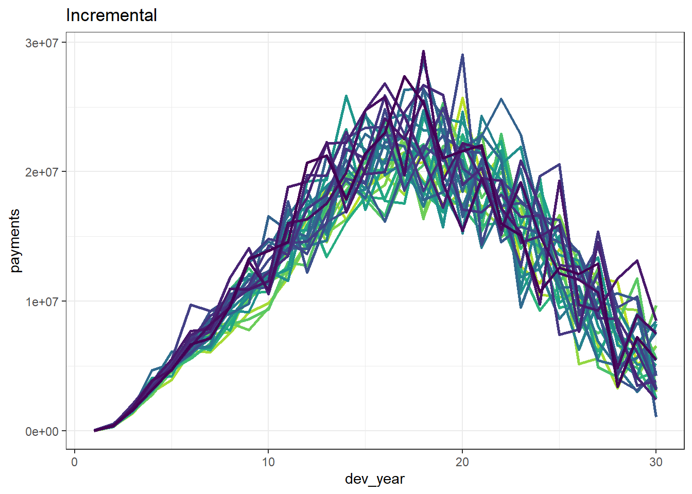
cum_paid_data = NULL

for (i in 1 : 30) {


  obj = paid_data$payments[paid_data$acc_year == i]
  obj = cumsum(obj)
  obj = data.frame(acc_year = i, dev_year = 1:(30) , cumulative = obj)
  cum_paid_data = rbind(cum_paid_data , obj)

}

p2 <- ggplot(data=cum_paid_data, aes(x=dev_year, y=cumulative, colour=as.factor(acc_year))) +  # Plot

  geom_line(linewidth=1) +
  scale_color_viridis_d(begin=0.9, end=0) +
  ggtitle("Cumulative") +
  theme_bw() +
  theme(legend.position = "bottom", legend.title=element_blank(), legend.text=element_text(size=6))

p2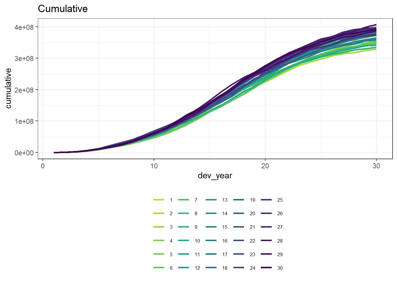
We can see that our dataset is quite homogeneous and has a clear inflationary trend.
Reserving with GLMs
Before we start looking at any machine learning techniques we will cover the blog on reserving with GLMs. Since many machine learning techniques are based on GLMs this is a good place to start. I also found it useful as a good place to re-familiarise myself with using R, while having a previous understanding of the underlying maths. Finally, using GLMs on unedited triangle data produces the same reserves as using a volume weighted all chain-ladder estimate, therefore it is easy to check the results being produced by R are what you expect.
If you are unsure of how GLMs work, I found the 2016 CAS monograph referenced in the GLM blog very useful. I’ve also found this article, which is a good place to start from scratch.
Following the code in the GLM blog is relatively simple. It begins with how the data is downloaded; this can be ignored as we don’t use it. Instead we will link in our SPLICE dataset as a data table and filter it for past values. We also load (or install) a number of packages.
library(data.table)  # manipulate the data
library(patchwork) # easily combine plots


options(scipen = 99)   # get rid of scientific notation

paid_data_GLM = data.table(paid_data)  # GLMs function requires data tables
paid_data_GLM = paid_data_GLM[paid_data_GLM$train_ind == TRUE] # set the data set for the GLM as the training data set only
Then we fit the model. Note we add a calender year factor, which the blog uses for diagnostics. Also we are using accf and devf as our factor names to agree with code in later blogs.
paid_data_GLM[, accf := as.factor(acc_year)  # GLMs require factors not numbers
                                            # Note we are using 'accf' and 'devf' as our factor names to agree with code in later blogs
][, devf := as.factor(dev_year)

][, cal_year := acc_year + dev_year - 1]

glm_fit1 <- glm(data = paid_data_GLM,

                family = quasipoisson(link = "log"),

                formula = "payments ~ 0 + accf + devf")


glm_fit1$coeff_table <- data.table(parameter = names(glm_fit1$coefficients),

                                   coeff_glm_fit1 = glm_fit1$coefficients)

head(glm_fit1$coeff_table)
parameter coeff_glm_fit1
1: accf1 9.579442
2: accf2 9.459583
3: accf3 9.500844
4: accf4 9.540363
5: accf5 9.518344
6: accf6 9.514399Next, we create a null dataset of future increments, to which we apply the GLM prediction, giving us our reserve estimate. This is achieved by following the code in the underlying blog, and is summarised in the table below.
# first make the lower triangle data set
ay <- NULL
dy <- NULL

for(i in 2:30){

  ay <- c(ay, rep(i, times=(i-1)))
  dy <- c(dy, (30-i+2):30)

}

futdata <- data.table(acc_year = ay, dev_year = dy)

# make factors
futdata[, cal_year := acc_year + dev_year
        ][, accf := as.factor(acc_year)
            ][, devf := as.factor(dev_year)]

# make the prediction and sum by acc_year
x <- predict(glm_fit1, newdata = futdata, type="response")

futdata[, incremental := x]

# data.table syntax to get summary by accident year
ocl_year <- futdata[,  lapply(.SD, sum), .SDcols=c("incremental"), by="acc_year"]

# total ocl
ocl_total <- futdata[, sum(incremental)]

# print the acc year table with total
ocl_year[, acc_year := as.character(acc_year) ]  # to make a table with total row
ocl_year_print <- rbind(ocl_year, data.table(acc_year="Total", incremental=ocl_total))
setnames(ocl_year_print, "incremental", "OCL")  # rename column for printing
datatable(ocl_year_print)|> formatRound("OCL", digits = 0)
As a check, I am going to see if my reserve matches the chain ladder method (which they should unless one of the leading diagonal payments is zero). The code is taken from the LASSO blog, introduced below, edited to fit the column names in our dataset and to perform a volume weighted all chain ladder.
# get cumulative payments to make it easier to calculate CL factors
paid_data_GLM[, cumpmts := cumsum(payments), by=.(acc_year)][train_ind==FALSE, cumpmts := NA]

cl_fac <- numeric(29) # hold CL factors for number of years we require reserves

for (j in 1:29){  # Code edited to be a volume weighted average on all years
  cl_fac[j] <-
    paid_data_GLM[train_ind==TRUE & dev_year == (j+1) & acc_year <= (30-j), sum(cumpmts)] /
    paid_data_GLM[train_ind==TRUE & dev_year == (j) & acc_year <= (30-j), sum(cumpmts)]
}

# accumulate the CL factors
cl_cum <- rev(cumprod(rev(cl_fac)))

# leading diagonal for projection
leading_diagonal <- paid_data_GLM[train_ind==TRUE & acc_year + dev_year == 31 & acc_year > 1, cumpmts]

# CL amounts now
cl_os <- cl_cum * leading_diagonal - leading_diagonal

sum(cl_os) - ocl_year_print$OCL[30]
[1] 0.3830585The difference is essentially zero - rounding / floating point errors are likely the source of it not being exactly zero.
Results by accident year are shown below
cl_os = rev(cl_os)
cl_os[30] = sum(cl_os)

ocl_year_print$cl_os = cl_os

ocl_year_print$difference = ocl_year_print$cl_os - ocl_year_print$OCL

datatable(ocl_year_print )|> formatRound(c("OCL", "cl_os"), digits = 0) |> formatRound("difference", digits = 4)
The GLM blog also gives a number of ways of performing diagnostics on the model, in order to refine it, for example by reducing overfitting or incorporating interaction terms. I won’t go into this in detail as it is standard GLM work and is also fairly complex, especially when using your own data set.
Reserving with LASSO
The next blog describes our first Machine Learning technique Self-assembling claim reserving models using the LASSO. LASSO stands for Least Absolute Shrinkage and Selection Operator. It is a ‘regularised regression’ method which acts like a GLM (as described in the previous section) but penalises the use of additional features and hence complex models, by using basis functions (functions of acc, dev and cal). There is some detail on this in the LASSO blog under the Set of basis functions heading, however, it took me a little while to get my head around. After some googling I found this website to be useful.
The LASSO blog details some of the mathematics behind the model, which should be fairly simple to understand for anyone with a good knowledge of statistics, including the model selection sections which introduces Lambda - the hyperparameter for this model. A hyperparameter is a parameter whose value is used to control the learning process. It cannot be fitted by the data, rather needs to be tuned by assessing the value that optimizes the model’s speed and quality of learning process.
The blog then states the advantages of the LASSO model, being an automatic method of dealing with data sets with complex features, such as shock inflationary events where chain ladder methods fail. GLMs are able to do this, but the design can be very time consuming. The LASSO model has performed this well in general.
Again the LASSO blog then generates its own data set, which we can skip over, bringing in our own data set instead (which needs to be changed to a data table). However, we do need to load the glmnet package (this might need to be installed). We need to create another column in our data for calendar year, named cal (accident + development -1), and it would also be useful to change the other column names to match those used in the blog (pmts, acc and dev). Note I have also changed our dataset to the data table called dat to match the blog.
library(glmnet) Loading required package: MatrixLoaded glmnet 4.1-8# colour palette for some plots
# IFoA colours
# primary colours
dblue <- "#113458"
mblue <- "#4096b8"
gold <- "#d9ab16"
lgrey <- "#dcddd9"
dgrey <- "#3f4548"
black <- "#3F4548"
#secondary colours
red <- "#d01e45"
purple <- "#8f4693"
orange <- "#ee741d"
fuscia <- "#e9458c"
violet <- "#8076cf"
dat = paid_data # Change the name to fit with the blog code
colnames(dat) = c( "acc", "dev", "pmts","train_ind" ) # Change the columns to fit with the blog code
dat = cbind(dat , cal = dat$acc + dat$dev - 1 )
dat = data.table(dat) # change the format to a data table so the manipulation below worksBefore we start coding the basis functions, there is a note in the LASSO blog on scaling the basis functions, where each basis function is divided by a scaling factor. We calculate one scaling factor for each feature (i.e. accident, development or calendar period), and divide each basis function by the scaling factor that the function relates to. The scaling factors are determined by a simple formula that resembles a variance calculation. Scaling prevents the values of each basis function impacting the penalty against each parameter in the loss function, which should only be determined by Lambda.
The code first sets up the scaling parameters and then generates the basis functions. Note the use of the linear spline function, which is defined when creating the LASSO dataset that the LASSO blog is using. Since we have skipped this section, we have to go back to get this code before we generate our basis functions as well as defining the numperiods variable (in our case 30).
num_periods = 30 # Set to the number of periods in your data set

LinearSpline <- function(var, start, stop){
  pmin(stop - start, pmax(0, var - start))
}

GetScaling <- function(vec) {

  fn <- length(vec)
  fm <- mean(vec)
  fc <- vec - fm
  rho_factor <- ((sum(fc^2))/fn)^0.5
}

# function to create the ramps for a particular primary vector
GetRamps <- function(vec, vecname, np, scaling){

  # vec = fundamental regressor
  # vecname = name of regressor
  # np = number of periods
  # scaling = scaling factor to use
  # pre-allocate the matrix to hold the results for speed/efficiency

  n <- length(vec)
  nramps <- (np-1)

  mat <- matrix(data=NA, nrow=n, ncol=nramps)
  cnames <- vector(mode="character", length=nramps)

  col_indx <- 0

  for (i in 1:(np-1)){

    col_indx <- col_indx + 1
    mat[, col_indx] <- LinearSpline(vec, i, 999) / scaling
    cnames[col_indx] <- paste0("L_", i, "_999_", vecname)
  }
  colnames(mat) <- cnames
  return(mat)
}

# create the step (heaviside) function interactions
GetInts <- function(vec1, vec2, vecname1, vecname2, np, scaling1, scaling2) {

  # vec1 = fundamental regressor 1
  # vec2 = fundamental regressor 2
  # vecname1 = name of regressor 1
  # vecname2 = name of regressor 2
  # np = number of periods
  # scaling1 = scaling factor to use for regressor 1
  # scaling2 = scaling factor to use for regressor 2
  # pre-allocate the matrix to hold the results for speed/efficiency

  n <- length(vec1)
  nints <- (np-1)*(np-1)

  mat <- matrix(data=NA_real_, nrow=n, ncol=nints)
  cnames <- vector(mode="character", length=nints)

  col_indx <- 0

  for (i in 2:np){

    ivec <- LinearSpline(vec1, i-1, i) / scaling1
    iname <- paste0("I_", vecname1, "_ge_", i)

    if (length(ivec[is.na(ivec)]>0)) print(paste("NAs in ivec for", i))

    for (j in 2:np){
      col_indx <- col_indx + 1
      mat[, col_indx] <- ivec * LinearSpline(vec2, j-1, j) / scaling2
      cnames[col_indx] <- paste0(iname, "xI_", vecname2, "_ge_", j)

      jvec <- LinearSpline(vec2, j-1, j) / scaling2

      if (length(jvec[is.na(jvec)]>0)) print(paste("NAs in jvec for", j))
    }
  }
  colnames(mat) <- cnames
  return(mat)
}
When setting up the scaling factors in ‘rho_factor_list’ I couldn’t get the for loop to work (something to do with the ‘get’ function), most likely due to my R skills. Instead of spending time sussing this out, I set the three scaling factors individually using the ‘GetScaling’ function.
# get the scaling values
rho_factor_list <- vector(mode="list", length=3)
names(rho_factor_list) <- c("acc", "dev", "cal")

rho_factor_list[["acc"]] = GetScaling(dat[dat$train_ind == TRUE, acc]) # I could not get the 'base::get()' function to work hence have split this into 3 lines
rho_factor_list[["dev"]] = GetScaling(dat[dat$train_ind == TRUE, dev])
rho_factor_list[["cal"]] = GetScaling(dat[dat$train_ind == TRUE, cal])
Once this has been done it should be trivial to set up our scaled basis functions and calculate the effects from our triangle, which is then stored in ‘varset’. We then drop any interaction columns that are constant e.g. columns involving future periods; these won’t affect the model but dropping them is good practice and makes the model run faster.
# main effects - matrix of values of Ramp functions

main_effects_acc <- GetRamps(vec = dat[, acc], vecname = "acc", np = num_periods, scaling = rho_factor_list[["acc"]])
main_effects_dev <- GetRamps(vec = dat[, dev], vecname = "dev", np = num_periods, scaling = rho_factor_list[["dev"]])
main_effects_cal <- GetRamps(vec = dat[, cal], vecname = "cal", np = num_periods, scaling = rho_factor_list[["cal"]])

main_effects <- cbind(main_effects_acc, main_effects_dev, main_effects_cal)

# interaction effects

int_effects <- cbind(
  GetInts(vec1=dat[, acc], vecname1="acc", scaling1=rho_factor_list[["acc"]], np=num_periods,
          vec2=dat[, dev], vecname2="dev", scaling2=rho_factor_list[["dev"]]),

  GetInts(vec1=dat[, dev], vecname1="dev", scaling1=rho_factor_list[["dev"]], np=num_periods,
          vec2=dat[, cal], vecname2="cal", scaling2=rho_factor_list[["cal"]]),

  GetInts(vec1=dat[, acc], vecname1="acc", scaling1=rho_factor_list[["acc"]], np=num_periods,
          vec2=dat[, cal], vecname2="cal", scaling2=rho_factor_list[["cal"]])
)

varset <- cbind(main_effects, int_effects)

# drop any constant columns over the training data set
# do this by identifying the constant columns and dropping them
# get the past data subset only using TRUE/FALSE from train_ind in dat

varset_train <- varset[dat$train_ind, ]

# identify constant columns as those with max=min

rm_cols <- varset_train[, apply(varset_train, MARGIN=2, function(x) max(x, na.rm = TRUE) == min(x, na.rm = TRUE))]

# drop these constant columns
varset <- varset[, !(colnames(varset) %in% colnames(rm_cols))]
Finally we come to fitting the model, using the cv.glmnet function, which is defined well in the LASSO blog, and then plotting log(Lambda) against the Poisson deviance. This shows which Lambda produces the lowest deviance from the cross-validation test performed by the function and hence is the best model. Cross-validation is explained well in the next blog R: Machine Learning Triangles hence I will not go into it in detail here except to say it is the most common method of tuning hyperparameters. The graph shows the Lambda at which the minimum deviance is achieved and a larger Lambda one standard deviation away. The reason for the larger Lambda is that some people view it as a good compromise between a model fitting well and possible overfit at the lambda.min model.
Note I have increased the maxit max iterations to 500,000, since the Lasso was not converging. This does not have a huge impact on the time it takes to run.
my_pmax <- num_periods^2   # max number of variables ever to be nonzero
my_dfmax <- num_periods*10  #max number of vars in the model

time1 <- Sys.time()
cv_fit <- cv.glmnet(x = varset[dat$train_ind,],
                    y = dat[train_ind==TRUE, pmts],
                    family = "poisson",
                    nlambda = 200,  # default is 100 but often not enough for this type of problem
                    nfolds = 8,
                    thresh = 1e-08, # default is 1e-7 but we found we needed to reduce it from time to time
                    lambda.min.ratio = 0, # allow very small values in lambda
                    dfmax = my_dfmax,
                    pmax = my_pmax,
                    alpha = 1,
                    standardize = FALSE,
                    maxit = 500000)  # convergence can be slow so increase max number of iterations

print("time taken for cross validation fit: ")
[1] "time taken for cross validation fit: "Sys.time() - time1 Time difference of 41.5844 secsplot(cv_fit) 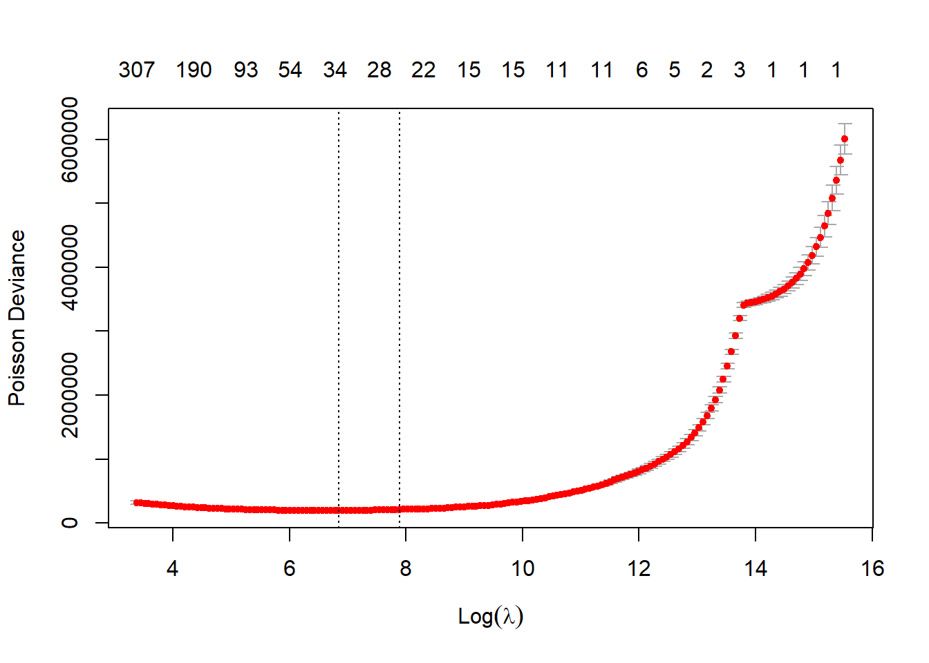
cv_fit$lambda.min [1] 945.3654cv_fit$lambda.1se [1] 2678.311The LASSO blog gives a couple of ways of assessing the appropriateness of the model; I will not go into these now as we will be carrying out a full model validation exercise in the next section. However, we do need the first bit of code in this section to fit the predicted values that the model gives us. Note if you do carry out this exercise the LASSO blog has an underlying ‘mu’ value in the data, which we don’t have and needs to be removed from the graph function.
Now we are ready to produce some reserves using the LASSO, and compare them to the chain ladder/GLM reserves. The code in the blog contains the code for the chain ladder reserves which we used above, hence we will not repeat it. The blog also produces a comparison plot and a summary of the outstanding reserves for each method.
dat[, fitted := as.vector(predict(cv_fit,
                                  newx = varset,
                                  s = cv_fit$lambda.min,
                                  type="response"))]


dat_LASSO = copy(dat) # Define a separate object to keep the results for comparison later

os_acc <- dat[train_ind == FALSE, # Summarise the LASSO and simulated reserves by accident year
              .(LASSO = sum(fitted), simulated = sum(pmts)), #Note we have removed the 'underlying' as this does not exist in our data
              keyby=.(acc)]

os <- os_acc[, .(LASSO = sum(LASSO), # Create totals
                 simulated = sum(simulated))]

# Add the CL amounts now

os_acc[, Chainladder := cl_os[-30]] # note we have already reversed the order of our chainladder reserves so do not need to here, need to remove the total we added
os[, Chainladder := sum(cl_os)]


# make a long [tidy format] version of the data for use with ggplot2
os_acc_long <- melt(os_acc, id.vars = "acc")

# divide by Bn to make numbers more readable

os_plot <-
  ggplot(data=os_acc_long, aes(x=acc, y=value, colour=variable,
                               linetype=variable, size=variable, alpha=variable))+
  geom_line()+
  scale_linetype_manual(name="", values=c("solid", "dashed", "dotted", "solid" ))+
  scale_colour_manual(name="", values=c(red, dgrey, dgrey, mblue ))+
  scale_size_manual(name="", values=c(2, 1, 1, 1.5))+
  scale_alpha_manual(name="", values=c(0.8, 0.5, 0.5, 0.8))+
  theme_classic()+
  theme(legend.position="bottom", legend.title=element_blank())+
  labs(x="Accident quarter", y="Amount")+
  ggtitle("Outstanding amounts")

os_plot
Warning: Using `size` aesthetic for lines was deprecated in ggplot2 3.4.0.
ℹ Please use `linewidth` instead.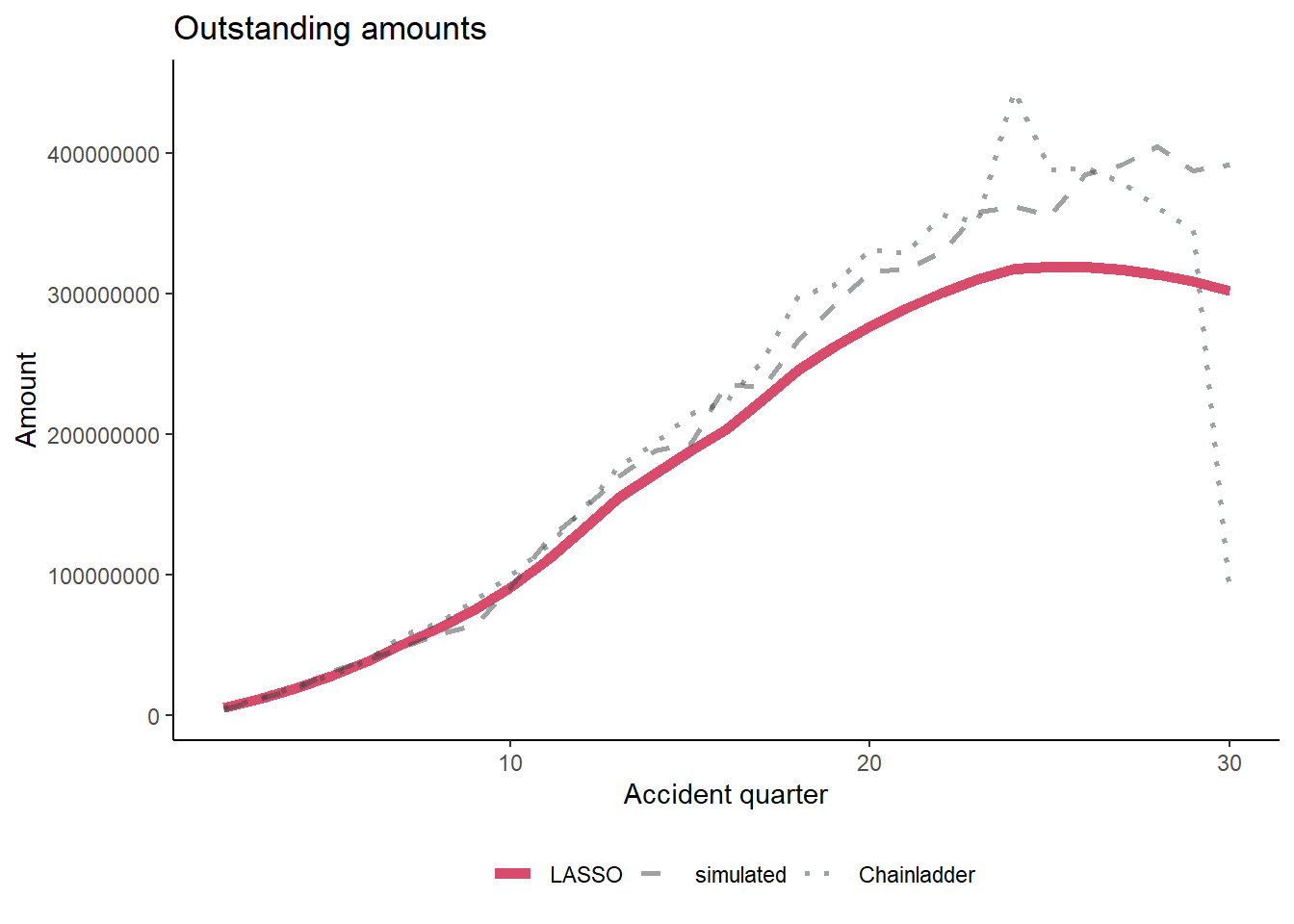
We discuss the effectiveness of the LASSO model at predicting the future reserves at the end of this blog, so I won’t comment on it now.
Machine Learning Triangles
The next blog brings together everything we’ve done so far, and compares a number of machine learning and non-machine learning methods:
- GLM
- LASSO
- Decision trees
- Random Forest
- XGBoost
It predominantly uses the mlr3 R package, which requires a number of packages that are shown in the MLT blog, so these need to be installed. The “mlr3extralearners” package is not on CRAN, but the blog provides code for this to be installed. R will ask you “Enter one or more numbers, or an empty line to skip updates”. Enter 1 in the Console and press enter to install all the updates. Note that the mlr3 package is constantly being developed so the version installed needs to be checked.
The MLT blog is focused on setting up data (which we don’t need to worry about as we will use our own), applying ML models to the data, tuning the hyperparameters and comparing the performance of the models.
When loading our data we can use the same code as for the LASSO model. However, note that we do need to set the accident and development years as factors and we want to label our rows 1:900.
library(mlr3)   # base mlr3 package
library(mlr3learners)  # implements common learners
library(mlr3tuning)    # tuning methodology
Loading required package: paradoxlibrary(paradox) # used to create parameter sets for hyperparameter tuning
library(mlr3extralearners) # needed for glms
library(rpart.plot) # to draw decision trees created by rpart Loading required package: rpart# ensure these packages are installed - but you don't need to attach them in the library command
# raprt
# ranger
# xgboost
# Reset our data
dat = paid_data # Change the name to fit with the blog code
colnames(dat) = c( "acc", "dev", "pmts", "train_ind" ) # Change the columns to fit with the blog code
dat = cbind(dat , cal = dat$acc + dat$dev - 1 )
dat = data.table(dat) # change the format to a data table so the manipulation below works
# create the num_periods variable - number of acc/dev periods
num_periods <- dat[, max(acc)]
dat[, accf := as.factor(acc)]
dat[, devf := as.factor(dev)]
# data.table code, .N = number of rows
dat[, row_id := 1:.N] We then set up an mlr3 task, which holds the data and sets roles for the data. When doing this, note that when setting new rules for the future data, you need to define the roles as “holdout” instead of “validation”, as there has been a change to the mlr3 package since the MLT blog was written.
# note can also use the sugar function tsk()
task <- TaskRegr$new(id = "reserves",
                     backend = dat[, .(pmts, train_ind, acc, dev, cal, row_id)],
                     target = "pmts")
We then set the training dataset “use” and the validation dataset “holdout”.
task$set_row_roles(dat[train_ind==FALSE, row_id], roles = "holdout")

# make row_id a name
task$set_col_roles("row_id", roles="name")

# drop train_ind from the feature list
task$col_roles$feature <- setdiff(task$feature_names, "train_ind")

# check the task has the correct variables now
task
<TaskRegr:reserves> (465 x 4)
* Target: pmts
* Properties: -
* Features (3):
- dbl (3): acc, cal, dev# check alll the col_roles
print(task$col_roles) $feature
[1] "acc" "cal" "dev"
$target
[1] "pmts"
$name
[1] "row_id"
$order
character(0)
$stratum
character(0)
$group
character(0)
$weight
character(0)As mentioned in the previous section of this blog, we now come on to how to tune the hyperparameters of a machine learning model, using cross-validation. A simple summary of cross-validation is it splits up the data we are using for fitting the model (i.e. the historic triangle data) into a training data set and a test data set. This split is done by splitting the data into K partitions and fitting the model to the data in all bar one of these partitions, and let the partition we left out be the test data set. We then repeat the process K times so that each partition is the test data set once. We then calculate then performance of the fitted model on each test set and average the performance. For this we need a performance measure, which will be the root mean square error (RMSE) here. We compare the average performance of fitted models with a variety of hyperparameters, to determine the optimum hyperparameters. There is a more detailed description of this in the MLT blog, but hopefully this description will make it easier to follow.
Setting up the cross-validation in mlr3 is very simple, and is done below. The MLT blog uses 6 folds (partitions) of the data and 25 evaluations (the number of different hyperparameter combinations to test).
# create object
crossval = rsmp("cv", folds=6)

set.seed(42)  # reproducible results

# populate the folds
# NB: mlr3 will only use data where role was set to “use”
crossval$instantiate(task)

# Setthe performance measure to root mean square error
measure <- msr("regr.rmse")
evals_trm = trm("evals", n_evals = 25)
Now it’s time to set up the decision tree, random forest and XGBoost models. The MLT blog doesn’t go into great detail about how these models work, so I have sourced some useful resources from a quick Google:
We now set up the decision tree, using the mlr3 and rpart.plot packages. The coding and theory behind decision trees are fairly simple:
# create a learner, ie a container for a decision tree model
lrn_rpart_default <- lrn("regr.rpart")

# fit the model on all the past data (ie where row_roles==use)
lrn_rpart_default$train(task)

# Visualise the tree
rpart.plot::rpart.plot(lrn_rpart_default$model, roundint = FALSE) 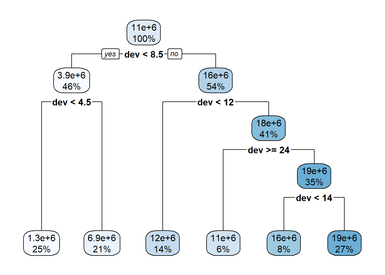
lrn_rpart_default$param_set <ParamSet>
id class lower upper nlevels default value
1: cp ParamDbl 0 1 Inf 0.01
2: keep_model ParamLgl NA NA 2 FALSE
3: maxcompete ParamInt 0 Inf Inf 4
4: maxdepth ParamInt 1 30 30 30
5: maxsurrogate ParamInt 0 Inf Inf 5
6: minbucket ParamInt 1 Inf Inf <NoDefault[3]>
7: minsplit ParamInt 1 Inf Inf 20
8: surrogatestyle ParamInt 0 1 2 0
9: usesurrogate ParamInt 0 2 3 2
10: xval ParamInt 0 Inf Inf 10 0However, tuning the hyperparameters of the tree is more involved, using the R library - paradox. The MLT blog shows you how to tune the complexity parameter cp and the minimum number of splits minsplits. The complexity parameter states the minimum improvement in RMSE that a model requires to add a node, as a result controls the complexity, speed and overfitting of the model. The code defines a range of complexity and minimum splits and tests 25 combinations of parameters within this range, producing the one with the lowest RMSE.
tune_ps_rpart <- ps(
  cp = p_dbl(lower = 0.001, upper = 0.1), # set the cp
  minsplit = p_int(lower = 1, upper = 10) # set the minsplit
)

# to see what's searched if we set a grid of 5
# rbindlist(generate_design_grid(tune_ps_rpart, 5)$transpose())

# create the hyper-parameter for this particular learner/model
instance_rpart <- TuningInstanceSingleCrit$new(

  task = task,
  learner = lrn("regr.rpart"),
  resampling = crossval,
  measure = measure,
  search_space = tune_ps_rpart,
  terminator = evals_trm
)

# create a grid-search tuner for a 5-point grid
tuner <- tnr("grid_search", resolution = 5)

# suppress log output for readability
lgr::get_logger("bbotk")$set_threshold("warn")
lgr::get_logger("mlr3")$set_threshold("warn")

tuner$optimize(instance_rpart)
cp minsplit learner_param_vals x_domain regr.rmse
1: 0.001 10 <list[3]> <list[2]> 1855345# restart log output
lgr::get_logger("bbotk")$set_threshold("info")
lgr::get_logger("mlr3")$set_threshold("info")
print(instance_rpart$result_learner_param_vals) $xval
[1] 0
$cp
[1] 0.001
$minsplit
[1] 10lrn_rpart_tuned <- lrn("regr.rpart")
lrn_rpart_tuned$param_set$values = instance_rpart$result_learner_param_vals
lrn_rpart_tuned$train(task)
# plot the model
rpart.plot::rpart.plot(lrn_rpart_tuned$model, roundint = FALSE) 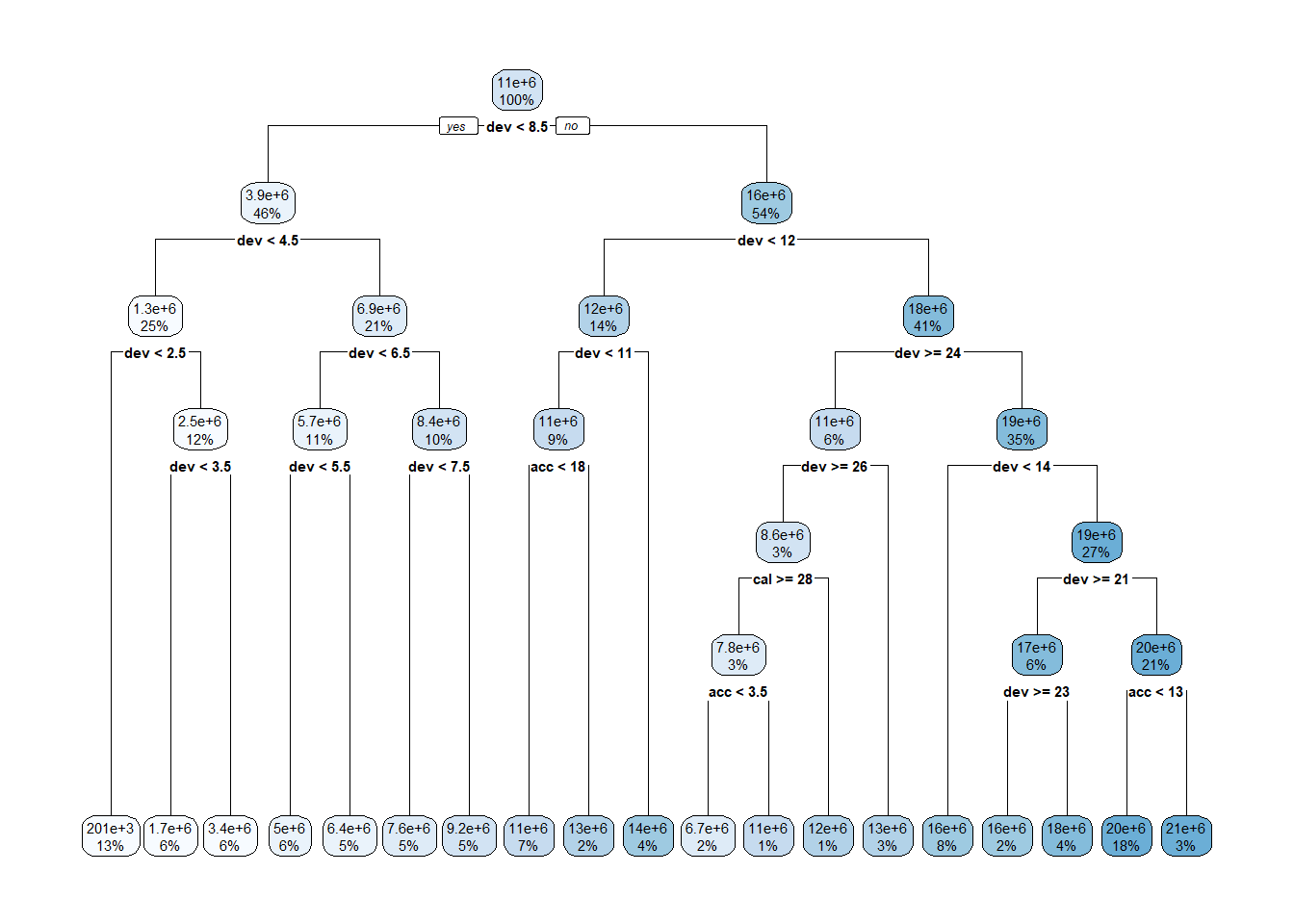
As noted in the MLT blog, decision trees are fairly poor models for our purposes but are a good introduction to mlr3 and tuning hyperparameters. There are plenty of other hyperparameters that can be tuned (many of which are mentioned in the link above), however, these are unlikely to help us much.
Setting up and tuning the random forest model is very similar. This time we will be tuning the number of trees and minimum node size (minimum number of splits for the decision trees in the forest) hyperparameters. mlr3 finds the best fit for the hyperparameters and then the blog fits rest of the hyperparameters for the model and outputs them.
# Random Forest
lrn("regr.ranger")$param_set
<ParamSet>
id class lower upper nlevels default
1: alpha ParamDbl -Inf Inf Inf 0.5
2: always.split.variables ParamUty NA NA Inf <NoDefault[3]>
3: holdout ParamLgl NA NA 2 FALSE
4: importance ParamFct NA NA 4 <NoDefault[3]>
5: keep.inbag ParamLgl NA NA 2 FALSE
6: max.depth ParamInt 0 Inf Inf
7: min.node.size ParamInt 1 Inf Inf 5
8: min.prop ParamDbl -Inf Inf Inf 0.1
9: minprop ParamDbl -Inf Inf Inf 0.1
10: mtry ParamInt 1 Inf Inf <NoDefault[3]>
11: mtry.ratio ParamDbl 0 1 Inf <NoDefault[3]>
12: num.random.splits ParamInt 1 Inf Inf 1
13: num.threads ParamInt 1 Inf Inf 1
14: num.trees ParamInt 1 Inf Inf 500
15: oob.error ParamLgl NA NA 2 TRUE
16: quantreg ParamLgl NA NA 2 FALSE
17: regularization.factor ParamUty NA NA Inf 1
18: regularization.usedepth ParamLgl NA NA 2 FALSE
19: replace ParamLgl NA NA 2 TRUE
20: respect.unordered.factors ParamFct NA NA 3 ignore
21: sample.fraction ParamDbl 0 1 Inf <NoDefault[3]>
22: save.memory ParamLgl NA NA 2 FALSE
23: scale.permutation.importance ParamLgl NA NA 2 FALSE
24: se.method ParamFct NA NA 2 infjack
25: seed ParamInt -Inf Inf Inf
26: split.select.weights ParamUty NA NA Inf
27: splitrule ParamFct NA NA 3 variance
28: verbose ParamLgl NA NA 2 TRUE
29: write.forest ParamLgl NA NA 2 TRUE
id class lower upper nlevels default
parents value
1: splitrule
2:
3:
4:
5:
6:
7:
8:
9: splitrule
10:
11:
12: splitrule
13: 1
14:
15:
16:
17:
18:
19:
20:
21:
22:
23: importance
24:
25:
26:
27:
28:
29:
parents valuetune_ps_ranger <- ps(
num.trees = p_int(lower = 100, upper = 900),
min.node.size = p_int(lower = 1, upper = 5)
)
# to see what's searched if we set a grid of 5
#rbindlist(generate_design_grid(tune_ps_ranger, 5)$transpose())
instance_ranger <- TuningInstanceSingleCrit$new(
task = task,
learner = lrn("regr.ranger"),
resampling = crossval,
measure = measure,
search_space = tune_ps_ranger,
terminator = evals_trm
)
# suppress output
lgr::get_logger("bbotk")$set_threshold("warn")
lgr::get_logger("mlr3")$set_threshold("warn")
#We can reuse the tuner we set up for the decision tree
#this was tuner <- tnr("grid_search", resolution = 5)
tuner$optimize(instance_ranger) num.trees min.node.size learner_param_vals x_domain regr.rmse
1: 700 1 <list[3]> <list[2]> 1678458# turn output back on
lgr::get_logger("bbotk")$set_threshold("info")
lgr::get_logger("mlr3")$set_threshold("info")
instance_ranger$result_learner_param_vals $num.threads
[1] 1
$num.trees
[1] 700
$min.node.size
[1] 1# Fit the model to all the parameters
lrn_ranger_tuned <- lrn("regr.ranger")
lrn_ranger_tuned$param_set$values = instance_ranger$result_learner_param_vals
lrn_ranger_tuned$train(task)
lrn_ranger_tuned$model Ranger result
Call:
ranger::ranger(dependent.variable.name = task$target_names, data = task$data(), case.weights = task$weights$weight, num.threads = 1L, num.trees = 700L, min.node.size = 1L)
Type: Regression
Number of trees: 700
Sample size: 465
Number of independent variables: 3
Mtry: 1
Target node size: 1
Variable importance mode: none
Splitrule: variance
OOB prediction error (MSE): 2887242432235
R squared (OOB): 0.9447452 Next, we set up the XGBoost model. Of all the models I’d recommend doing more research into this one. It was first designed in 2016 and has since taken the machine learning world by storm and hence is worth paying particular attention to. Similar to the decision tree and random forest we will be setting a few, but not all of the parameters. There are many more hyperparameters available to tune in the XGBoost model than the previous two, hence properly fitting one of these models will require more research. Here is a summary of the hyperparameters:
lrn("regr.xgboost")$param_set<ParamSet>
id class lower upper nlevels default
1: alpha ParamDbl 0 Inf Inf 0
2: approxcontrib ParamLgl NA NA 2 FALSE
3: base_score ParamDbl -Inf Inf Inf 0.5
4: booster ParamFct NA NA 3 gbtree
5: callbacks ParamUty NA NA Inf <list[0]>
6: colsample_bylevel ParamDbl 0 1 Inf 1
7: colsample_bynode ParamDbl 0 1 Inf 1
8: colsample_bytree ParamDbl 0 1 Inf 1
9: disable_default_eval_metric ParamLgl NA NA 2 FALSE
10: early_stopping_rounds ParamInt 1 Inf Inf
11: eta ParamDbl 0 1 Inf 0.3
12: eval_metric ParamUty NA NA Inf rmse
13: feature_selector ParamFct NA NA 5 cyclic
14: feval ParamUty NA NA Inf
15: gamma ParamDbl 0 Inf Inf 0
16: grow_policy ParamFct NA NA 2 depthwise
17: interaction_constraints ParamUty NA NA Inf <NoDefault[3]>
18: iterationrange ParamUty NA NA Inf <NoDefault[3]>
19: lambda ParamDbl 0 Inf Inf 1
20: lambda_bias ParamDbl 0 Inf Inf 0
21: max_bin ParamInt 2 Inf Inf 256
22: max_delta_step ParamDbl 0 Inf Inf 0
23: max_depth ParamInt 0 Inf Inf 6
24: max_leaves ParamInt 0 Inf Inf 0
25: maximize ParamLgl NA NA 2
26: min_child_weight ParamDbl 0 Inf Inf 1
27: missing ParamDbl -Inf Inf Inf NA
28: monotone_constraints ParamUty NA NA Inf 0
29: normalize_type ParamFct NA NA 2 tree
30: nrounds ParamInt 1 Inf Inf <NoDefault[3]>
31: nthread ParamInt 1 Inf Inf 1
32: ntreelimit ParamInt 1 Inf Inf
33: num_parallel_tree ParamInt 1 Inf Inf 1
34: objective ParamUty NA NA Inf reg:squarederror
35: one_drop ParamLgl NA NA 2 FALSE
36: outputmargin ParamLgl NA NA 2 FALSE
37: predcontrib ParamLgl NA NA 2 FALSE
38: predictor ParamFct NA NA 2 cpu_predictor
39: predinteraction ParamLgl NA NA 2 FALSE
40: predleaf ParamLgl NA NA 2 FALSE
41: print_every_n ParamInt 1 Inf Inf 1
42: process_type ParamFct NA NA 2 default
43: rate_drop ParamDbl 0 1 Inf 0
44: refresh_leaf ParamLgl NA NA 2 TRUE
45: reshape ParamLgl NA NA 2 FALSE
46: sample_type ParamFct NA NA 2 uniform
47: sampling_method ParamFct NA NA 2 uniform
48: save_name ParamUty NA NA Inf
49: save_period ParamInt 0 Inf Inf
50: scale_pos_weight ParamDbl -Inf Inf Inf 1
51: seed_per_iteration ParamLgl NA NA 2 FALSE
52: skip_drop ParamDbl 0 1 Inf 0
53: strict_shape ParamLgl NA NA 2 FALSE
54: subsample ParamDbl 0 1 Inf 1
55: top_k ParamInt 0 Inf Inf 0
56: training ParamLgl NA NA 2 FALSE
57: tree_method ParamFct NA NA 5 auto
58: tweedie_variance_power ParamDbl 1 2 Inf 1.5
59: updater ParamUty NA NA Inf <NoDefault[3]>
60: verbose ParamInt 0 2 3 1
61: watchlist ParamUty NA NA Inf
62: xgb_model ParamUty NA NA Inf
id class lower upper nlevels default
parents value
1:
2:
3:
4:
5:
6:
7:
8:
9:
10:
11:
12:
13: booster
14:
15:
16: tree_method
17:
18:
19:
20: booster
21: tree_method
22:
23:
24: grow_policy
25:
26:
27:
28:
29: booster
30: 1
31: 1
32:
33:
34:
35: booster
36:
37:
38:
39:
40:
41: verbose
42:
43: booster
44:
45:
46: booster
47: booster
48:
49:
50:
51:
52: booster
53:
54:
55: booster,feature_selector
56:
57: booster
58: objective
59:
60: 0
61:
62:
parents valueIt should also be noted that we need a lot more evaluations to run XGBoost, and hence it takes a longer time to run. The MLT blog provides the code for modelling the XGBoost with any number of evaluations, as well as a best fit model, which had been previously developed. I am going to fit two models, one with 25 evaluations and one with 500, but not attempt a best fit model.
Editor’s note: since this code takes a while to run (~18 mins on a 6.5 year old computer), I haven’t rerun it here. The next code chunk below uses the results from this block of code to fit the two models, one tuned with the 25 evaluations and one from the 500.
tune_ps_xgboost <- ps(
    # ensure non-negative values
  objective = p_fct("reg:tweedie"),
  tweedie_variance_power = p_dbl(lower = 1.01, upper = 1.99),

  # eta can be up to 1, but usually it is better to use low eta, and tune nrounds for a more fine-grained model
  eta = p_dbl(lower = 0.01, upper = 0.3),

  # select value for gamma
  # tuning can help overfitting but we don't investigate this here
  gamma = p_dbl(lower = 0, upper = 0),

  # We know that the problem is not that deep in interactivity so we search a low depth
  max_depth = p_int(lower = 2, upper = 6),

  # nrounds to stop overfitting
  nrounds = p_int(lower = 100, upper = 500)
)

instance_xgboost <- TuningInstanceSingleCrit$new(

  task = task,
  learner = lrn("regr.xgboost"),
  resampling = crossval,
  measure = measure,
  search_space = tune_ps_xgboost,
  terminator = evals_trm
)

# need to make a new tuner with resolution 4
#tuner <- tnr("grid_search", resolution = 4)
set.seed(84)  # for random search for reproducibility
tuner <- tnr("random_search")

lgr::get_logger("bbotk")$set_threshold("warn")
lgr::get_logger("mlr3")$set_threshold("warn")

time_bef <- Sys.time()
tuner$optimize(instance_xgboost)

lgr::get_logger("bbotk")$set_threshold("info")
lgr::get_logger("mlr3")$set_threshold("info")

Sys.time() - time_bef

#500 evals
evals_trm2 = trm("evals", n_evals = 500)

tune_ps_xgboost_500 <- ps(

  # ensure non-negative values
  objective = p_fct("reg:tweedie"),
  tweedie_variance_power = p_dbl(lower = 1.01, upper = 1.99),

  # eta can be up to 1, but usually it is better to use low eta, and tune nrounds for a more fine-grained model
  eta = p_dbl(lower = 0.01, upper = 0.3),
  # select value for gamma
  # tuning can help overfitting but we don't investigate this here
  gamma = p_dbl(lower = 0, upper = 0),

  # We know that the problem is not that deep in interactivity so we search a low depth
  max_depth = p_int(lower = 2, upper = 6),

  # nrounds to stop overfitting
  nrounds = p_int(lower = 100, upper = 500)
)

instance_xgboost_500 <- TuningInstanceSingleCrit$new(

  task = task,
  learner = lrn("regr.xgboost"),
  resampling = crossval,
  measure = measure,
  search_space = tune_ps_xgboost_500,
  terminator = evals_trm2
)

# need to make a new tuner with resolution 4
#tuner <- tnr("grid_search", resolution = 4)
set.seed(84)  # for random search for reproducibility
tuner <- tnr("random_search")

lgr::get_logger("bbotk")$set_threshold("warn")
lgr::get_logger("mlr3")$set_threshold("warn")

time_bef <- Sys.time()
tuner$optimize(instance_xgboost_500)

lgr::get_logger("bbotk")$set_threshold("info")
lgr::get_logger("mlr3")$set_threshold("info")

Sys.time() - time_bef
We need to manually train our XGBoost models, by setting the hyperparameters.
If you’ve run the code above then you can see the parameters using this code:
instance_xgboost$result_learner_param_vals
instance_xgboost_500$result_learner_param_vals
Set the hyperparameters (using previously run tuning parameters if you haven’t rerun the code) and train the models:
lrn_xgboost_25 = lrn("regr.xgboost", objective="reg:tweedie", nrounds=192,
                     tweedie_variance_power=1.448514, eta=0.1726785, gamma=0, max_depth=3)
lrn_xgboost_25$train(task)

lrn_xgboost_500 = lrn("regr.xgboost", objective="reg:tweedie", nrounds=159,
                      tweedie_variance_power=1.138227, eta=0.07166036, gamma=0, max_depth=2)
lrn_xgboost_500$train(task)
Include XGBoost in our set of models:
# make a new copy of the data, deleting the row_id, accf and devf columns
model_forecasts <- copy(dat)[, c("row_id", "accf", "devf") := NULL]

# add the model projections - specify list of learners to use and their names
lrnrs <- c(lrn_rpart_tuned, lrn_ranger_tuned, lrn_xgboost_25, lrn_xgboost_500) #add 500

# the id property is used to name the variables - since we have 2 xgboosts, adjust id where necessary
lrn_xgboost_25$id <- "regr.xgboost_25"
lrn_xgboost_500$id <- "regr.xgboost_500"

for(l in lrnrs){

  #learner$predict(task, row_ids) is how to get predicted values, returns 3 cols with preds in response
  # use row_ids to tell it to use entire data set, ie "use" and validation rows
  #model_forecasts[, (nl) := l$predict(task, row_ids=1:nrow(dat))$response]
  model_forecasts[, l$id := l$predict(task=task, row_ids=1:nrow(dat))$response]

}
We then add our GLM estimate. In the MLT blog this is done with a new GLM, however, we can re-use ours.
# GLM
model_forecasts[, "regr.glm" := predict(glm_fit1, newdata=dat[, .(pmts, accf, devf)], type="response")]
Include our LASSO estimates in the model forecasts. The MLT blog shows how to use the mlr3 package to perform the LASSO model, but this is surplus to requirement here.
# Bring in LASSO results from before
model_forecasts$regr.cv_glmnet = dat_LASSO$fitted
Now it’s a case of comparing all the models. We calculate the RMSE and the standard error contribution of the training and test data and output a number of graphs so we can investigate our models.
# get list of variables to form observations by - this is why we used a common naming structure
model_names <- names(model_forecasts)[ names(model_forecasts) %like% "regr"]

# wide -> long
model_forecasts_long <- melt(model_forecasts,

                             measure.vars = model_names,
                             id.vars=c("acc", "dev", "cal", "pmts", "train_ind"))
setnames(model_forecasts_long, c("variable", "value"), c("model", "fitted"))

model_rmse <- model_forecasts_long[, se_contrib := (fitted-pmts)^2
][, .(se_contrib = sum(se_contrib), num = .N), by=.(model, train_ind)
][, rmse := sqrt(se_contrib / num)]

datatable(model_rmse) |> formatRound("se_contrib", digits = 0)|> formatRound("rmse", digits = 0)
We can see the XGBoost with 500 iterations has the lowest RMSE and the LASSO and decision tree being next on the future values, with the random forest performing the worst. This is interesting as the random forest has the lowest RMSE on the past values, which may show overfitting and not picking up the inflationary trend.
Let’s add in the actuals for comparison.
# add in the actual values for comparison
actuals <- model_forecasts_long[model=="regr.glm",]
actuals[, model := "actual"
][, fitted := pmts]

model_forecasts_long_plot <- rbind(actuals, model_forecasts_long)

# calculate log_fitted
model_forecasts_long_plot[, log_fitted := log(pmax(1, fitted))]
Our first diagnostic graphs give us a quick visual comparison of the fitted values compared to the actuals.
GraphHeatMap <- function(dat, x="dev", y="acc", facet="model", actual, fitted, lims=c(0.25, 4),
                         xlab="Development quarter", ylab="Accident Quarter"){
  # copy data to avoid modifying original
  localdat <- copy(dat)

  # get fails if there is a variable with the same name so make local copies
  local_x <- x
  local_y <- y
  local_actual <- actual
  local_fitted <- fitted

  np <- max(localdat[[y]])
  localdat[, .avsf := get(local_actual) / get(local_fitted)
  ][, .avsf_restrict_log := log(pmax(min(lims), pmin(max(lims), .avsf)))
  ][, .past_line := np + 1 - get(local_y)]

  g <- ggplot(data=localdat, aes_string(x=local_x, y=local_y)) +
    geom_tile(aes(fill = .avsf_restrict_log))+scale_y_reverse()+
    facet_wrap(~get(facet), ncol=2)+
    theme_classic()+
    scale_fill_gradient2(name="log(Acc vs Fit)", low=mblue, mid="white", high=red, midpoint=0, space="Lab", na.value="grey50", guide="colourbar")+
    labs(x=xlab, y=ylab)+
    geom_line(aes_string(x=".past_line", y=local_y), colour=dgrey, size=2)+
    theme(strip.text = element_text(size=8,colour="grey30"), strip.background = element_rect(colour="white", fill="white"))+
    theme(axis.title.x = element_text(size=8), axis.text.x  = element_text(size=7))+
    theme(axis.title.y = element_text(size=8), axis.text.y  = element_text(size=7))+
    theme(element_line(linewidth=0.25, colour="grey30"))+
      theme(legend.position="bottom",  legend.direction = "horizontal",  legend.text=element_text(size=6) ,  legend.title =element_text(size=8) )
    NULL

  invisible(list(data=localdat, graph=g))
}

g <- GraphHeatMap(model_forecasts_long, x="dev", y="acc", facet="model", actual="pmts", fitted="fitted")
g$graph 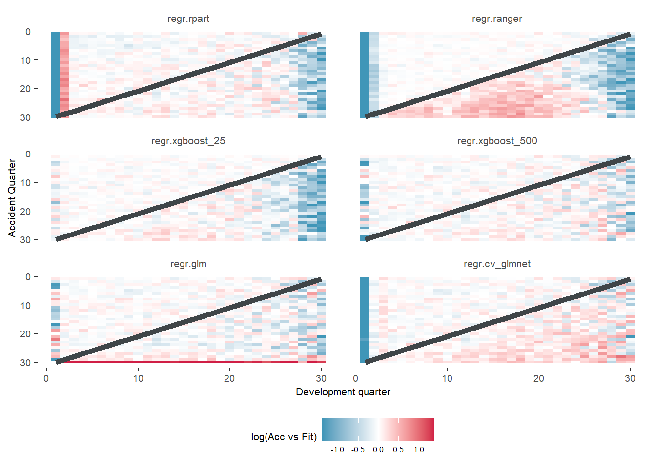
There are a couple of interesting observations here. We can see the random forest performs well for the history but not the future. The XGBoost_500 looks good in general. The LASSO model performs steadily worse we we go into the future. The XGBoost_25 also struggles to pick up the trend in the later development periods.
We can now look at a reserve predictions comparison.
# summarise the future payments and each model projection by accident quarter
# remember ml is a character vector of all the model names, which are columns of
#   fitted values in model_forecasts

# get reserves and payments by accident quarter
os_acc <- model_forecasts_long[train_ind == FALSE, .(actual=sum(pmts), reserve=sum(fitted)), by=.(model, acc)]

# make full tidy data set by stacking actuals
os_acc <- rbind(os_acc[model=="regr.glm",][, reserve := actual][, model := "actual"],
                os_acc)

setkey(os_acc, model, acc)

# create a factor variable from model so we can order it in the plot as we wish
g1 <- ggplot(data=os_acc, aes(x=acc, y=reserve, group=model)) +
  geom_line(aes(linetype=model, colour=model, size=model, alpha=model))+
  scale_colour_manual(name="", values=c(dgrey, red, dgrey, fuscia, dgrey, mblue, gold))+
  scale_linetype_manual(name="", values=c("solid", "solid", "dotted", "dotdash", "dashed", "longdash", "solid"))+
  scale_size_manual(name="", values=c(2.5, 2, 1, 1.25, 1, 1.25, 1.5))+
  scale_alpha_manual(name="", values=c(1, 0.9, 0.5, 0.7, 0.5, 0.7, 0.9))+
  coord_cartesian(ylim=c(0, 500000000), xlim=c(0, 40))+
  theme_classic() +
  theme(legend.position = "bottom")+
  labs(y="Reserve", x="Accident Quarter")+
  NULL

g1 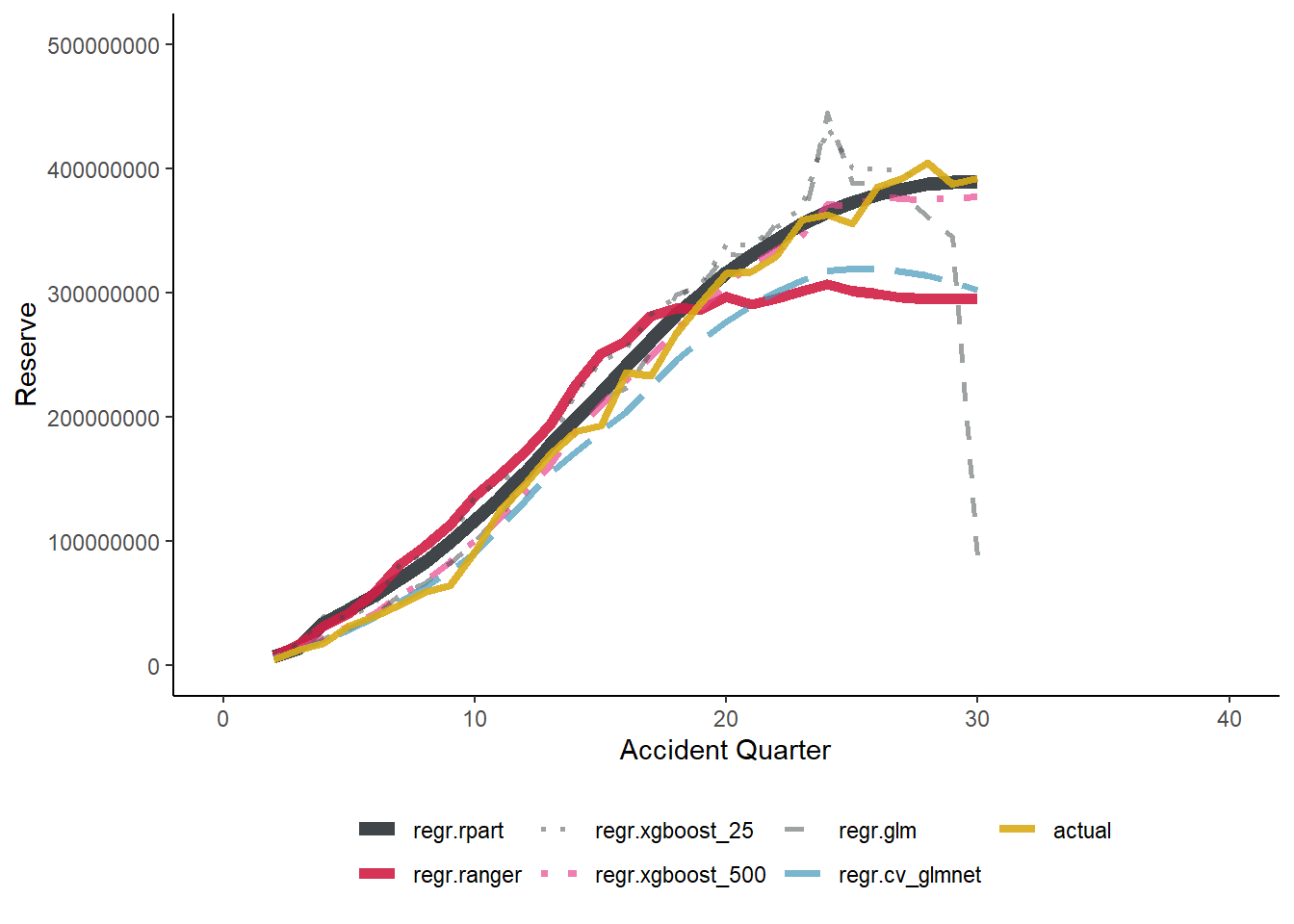
os <- os_acc[, .(reserve=sum(reserve), actual=sum(actual)), by=.(model)]
os[, ratio := reserve / actual][, actual := NULL]

# sort
os[, ratio_diff := abs(ratio-100)]
os <- os[order(ratio_diff)][, ratio_diff := NULL]

# output table
setnames(os, c("model", "reserve", "ratio"), c("Model", "Reserve", "Ratio to actual(%)"))
datatable(os)|> formatRound("Reserve", digits = 0)|> formatPercentage("Ratio to actual(%)")
We can see again the XGBoost performing really well here. Interestingly the GLM/Chain ladder performs well in terms of predicting reserves, but clearly there is an offsetting as it predicts very low reserves for later periods. The LASSO model and random forests under predicts the reserves in the later accident periods, showing they do not pick up on the inflationary trends adequately. It is interesting to note the relatively low RMSE for the LASSO when looking at these results, which could be reflective of the high performance of the model in earlier accident periods.
The decision tree forecast (rpart) performs surprisingly well on this data set. Based on anecdotal experience from this working party this is unusual.
The MLT blog also looks at a large number of other diagnostics which would be useful when assessing the model performance but I will let the reader do this independently.
Conclusion
I found working through these blogs and learning these techniques to be a tough but rewarding journey. Hopefully this blog will make the process easier for others looking to learn machine learning in reserving. However, this blog only covers the very beginnings of what the working party has produced and is researching. For example there are blogs that cover this material but in Python, if that is your preferred programming language. Furthermore there are blogs working through Neural Networks, ML model diagnostics and practical considerations for insurance companies.
Appendix
I have included a summary of all the links in this blog for completeness:
Working party material
Other useful resources
- Actuarial cookbook
- SPLICE
- DataCamp introduction to R
- CAS monograph on stochastic reserving
- GLMs
- Basis functions and regularisation
- Decision trees
- Random forests
- xgboost
Finally, here are details of the R session as well as commented out code to install the various packages
#install.packages("SPLICE")
#install.packages("DT")
#install.packages("data.table")  # manipulate the data
#install.packages("ggplot2")   # plot the data
#install.packages("viridis")   # plot colours that are friendly to colour blindness
#install.packages("patchwork") # easily combine plots
#install.packages("glmnet")
#install.packages("mlr3")
#install.packages("mlr3learners")
#install.packages("mlr3tuning")
#install.packages("paradox")
#install.packages("remotes")
#remotes::install_github("mlr-org/mlr3extralearners")
#install.packages("rpart.plot")
#install.packages("ranger")
#install.packages("xgboost")
sessionInfo()
R version 4.3.1 (2023-06-16 ucrt)
Platform: x86_64-w64-mingw32/x64 (64-bit)
Running under: Windows 10 x64 (build 19045)
Matrix products: default
locale:
[1] LC_COLLATE=English_Ireland.utf8 LC_CTYPE=English_Ireland.utf8
[3] LC_MONETARY=English_Ireland.utf8 LC_NUMERIC=C
[5] LC_TIME=English_Ireland.utf8
time zone: Europe/Dublin
tzcode source: internal
attached base packages:
[1] stats graphics grDevices datasets utils methods base
other attached packages:
[1] rpart.plot_3.1.1 rpart_4.1.16
[3] mlr3extralearners_0.5.49-9000 mlr3tuning_0.14.0
[5] paradox_0.10.0 mlr3learners_0.5.4
[7] mlr3_0.14.0 glmnet_4.1-8
[9] Matrix_1.5-4.1 patchwork_1.1.3
[11] ggplot2_3.4.4 data.table_1.14.8
[13] DT_0.30 SPLICE_1.1.1
[15] SynthETIC_1.0.5
loaded via a namespace (and not attached):
[1] tidyselect_1.1.2 viridisLite_0.4.1 dplyr_1.0.10
[4] farver_2.1.1 fastmap_1.1.1 digest_0.6.33
[7] lifecycle_1.0.3 survival_3.5-5 magrittr_2.0.3
[10] compiler_4.3.1 rlang_1.1.1 sass_0.4.2
[13] tools_4.3.1 utf8_1.2.2 yaml_2.3.7
[16] knitr_1.40 labeling_0.4.2 htmlwidgets_1.5.4
[19] xgboost_1.6.0.1 withr_2.5.0 purrr_0.3.5
[22] mlr3misc_0.11.0 grid_4.3.1 fansi_1.0.3
[25] mlr3measures_0.5.0 colorspace_2.0-3 future_1.28.0
[28] globals_0.16.1 scales_1.2.1 iterators_1.0.14
[31] cli_3.6.1 rmarkdown_2.16 crayon_1.5.2
[34] bbotk_0.5.4 generics_0.1.3 rstudioapi_0.14
[37] future.apply_1.9.1 DBI_1.1.3 cachem_1.0.6
[40] stringr_1.4.1 splines_4.3.1 assertthat_0.2.1
[43] parallel_4.3.1 vctrs_0.6.4 jsonlite_1.8.2
[46] listenv_0.8.0 crosstalk_1.2.0 foreach_1.5.2
[49] lgr_0.4.4 jquerylib_0.1.4 glue_1.6.2
[52] parallelly_1.32.1 codetools_0.2-19 stringi_1.7.8
[55] shape_1.4.6 gtable_0.3.1 palmerpenguins_0.1.1
[58] munsell_0.5.0 tibble_3.1.8 pillar_1.8.1
[61] htmltools_0.5.5 R6_2.5.1 evaluate_0.16
[64] lattice_0.21-8 backports_1.4.1 renv_1.0.3
[67] bslib_0.4.0 Rcpp_1.0.9 uuid_1.1-0
[70] checkmate_2.1.0 ranger_0.14.1 xfun_0.33
[73] pkgconfig_2.0.3